Center Alignment Index (CAI): A Novel Metric for Evaluating Data Center Agreement on the 1:1 Line
Introduction to Center Alignment Index (CAI) as a Regression Metric
1. Mathematical Definition and Components
The Center Alignment Index (CAI) is a bounded metric designed to quantify how closely the central tendency of paired observations aligns with the 1:1 identity line (y = x). In many scientific and engineering domains, comparing two measurement systems or model predictions against observed values requires assessing whether the data center (i.e., the bivariate mean) falls on the line of perfect agreement. CAI addresses this need by providing a single, unitless score ranging from 0 to 1.
1.1 The Formula
Given paired observations $(x_i, y_i)$ for $i = 1, 2, \ldots, n$, define the following sample statistics:
$$\mu_x = \frac{1}{n}\sum_{i=1}^{n} x_i, \quad \mu_y = \frac{1}{n}\sum_{i=1}^{n} y_i$$
$$\sigma_x = \sqrt{\frac{1}{n-1}\sum_{i=1}^{n}(x_i – \mu_x)^2}, \quad \sigma_y = \sqrt{\frac{1}{n-1}\sum_{i=1}^{n}(y_i – \mu_y)^2}$$
The location shift parameter is defined as:
$$u = \frac{\mu_x – \mu_y}{\sqrt{\sigma_x \cdot \sigma_y}}$$
The Center Alignment Index is then:
$$CAI = \frac{1}{1 + u^2}$$
The CAI curve can be made steeper or more gradual by introducing the tolerance parameter $k$:
$$CAI(u;\,k) = \frac{1}{1 + u^2 / k}$$
The parameter $k$ controls the half-power point: $CAI(u;\,k) = 0.5$ occurs at $u = \sqrt{k}$. A larger $k$ makes the metric more tolerant of bias; a smaller $k$ makes it stricter.
1.2 Decomposition
The CAI formula can be decomposed into three interpretable components:
Numerator (Bias Term): The raw bias $\mu_x – \mu_y$ captures the absolute difference between the means of the two variables. When $\mu_x = \mu_y$, the
data center lies exactly on the 1:1 line, and the numerator of $u$ becomes zero.
Denominator (Scale Normalizer): The geometric mean standard deviation $\sqrt{\sigma_x \cdot \sigma_y}$ serves as a natural scaling factor. This normalization ensures that the location shift $u$ is dimensionless, making CAI invariant to the measurement unit. Whether the data are in millimeters or kilometers, the CAI value remains the same.
Transformation Function: The mapping $f(u) = 1/(1 + u^2)$ is a Lorentzian (Cauchy kernel) function. This smooth, monotonically decreasing function of $|u|$ ensures that CAI transitions continuously from 1 (perfect alignment) toward 0 (complete misalignment) without any threshold discontinuities.
1.3 Physical Meaning
Geometrically, the data center $(\mu_x, \mu_y)$ is a single point in the scatter plot. The 1:1 line is defined by $y = x$. The perpendicular distance from the data center to this line is:
$$d = \frac{|\mu_y – \mu_x|}{\sqrt{2}}$$
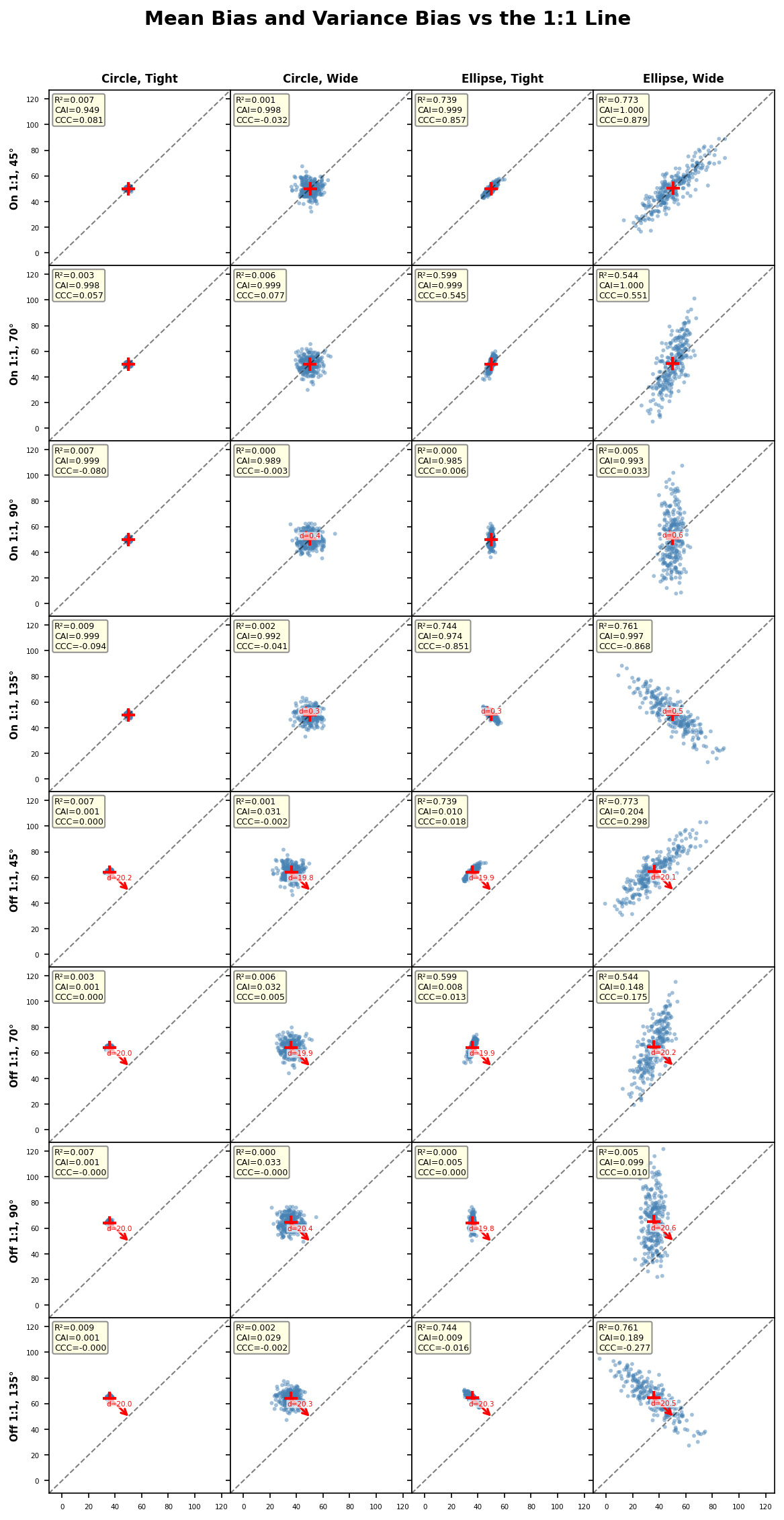
CAI translates this distance into a normalized agreement score. A CAI of 1.0 indicates that the bivariate mean sits exactly on the 1:1 line, implying zero systematic bias between the two variables. As the data center drifts away from the 1:1 line, CAI decreases toward zero. The rate of decrease depends on the intrinsic variability of the data: for highly variable data (large $\sigma_x$ and $\sigma_y$), the same absolute bias produces a smaller $u$ and thus a higher CAI, reflecting that the bias is relatively less important compared to the natural spread.
1.4 Relation to CCC
Lin’s Concordance Correlation Coefficient (CCC) is widely used to evaluate agreement between two continuous variables. CCC is defined as:
$$\rho_c = \frac{2\sigma_{xy}}{\sigma_x^2 + \sigma_y^2 + (\mu_x – \mu_y)^2}$$
Lin demonstrated that CCC can be decomposed multiplicatively:
$$\rho_c = r \times C_b$$
where $r$ is the Pearson correlation coefficient (precision) and $C_b$ is the bias correction factor (accuracy):
$$C_b = \frac{2}{v + \frac{1}{v} + u^2}, \quad v = \frac{\sigma_x}{\sigma_y}$$
The bias correction factor $C_b$ contains two components: the scale shift $v$ (ratio of standard deviations) and the location shift $u$ (normalized mean difference). CAI isolates the location shift component by fixing $v = 1$ (assuming equal scales), yielding:
$$C_b \big|_{v=1} = \frac{2}{2 + u^2} = \frac{1}{1 + u^2/2}$$
CAI adopts a slightly more aggressive penalization by using $1/(1 + u^2)$ rather than $1/(1 + u^2/2)$. This design choice makes CAI more sensitive to location shifts while completely decoupling it from scale differences. In practice, CAI serves as a pure location bias diagnostic that complements CCC by isolating whether the disagreement is due to a shifted center or due to other factors such as differential scaling or imprecision.
2. Interpretation of CAI Values
| CAI Range | Interpretation | Typical Scenario |
|---|---|---|
| 0.95 to 1.00 | Excellent center alignment | Near-zero systematic bias |
| 0.80 to 0.95 | Good alignment | Minor calibration offset present |
| 0.50 to 0.80 | Moderate misalignment | Noticeable bias requiring correction |
| 0.20 to 0.50 | Poor alignment | Substantial systematic bias |
| 0.00 to 0.20 | Very poor alignment | Fundamental disagreement between variables |
A practical guideline: when CAI drops below 0.80, it suggests that the systematic bias between two measurement systems or between predictions and
observations is large enough relative to the data variability that a simple additive correction (bias adjustment) should be considered before further analysis or model deployment.
It is important to note that CAI evaluates only the location of the data center. A high CAI does not guarantee that individual data points agree well; it only confirms that there is no systematic shift. Conversely, a low CAI pinpoints the presence of a mean-level discrepancy, which is often the first and most correctable source of disagreement.
3. Applications in AI/ML
- Model Validation: In machine learning, CAI can serve as a diagnostic tool during model evaluation. When comparing predicted values against ground truth, a CAI close to 1.0 confirms that the model does not exhibit systematic over- or under-prediction on average. This is especially useful for regression tasks in domains such as remote sensing, climate modeling, and medical imaging where systematic bias has practical consequences.
- Transfer Learning Diagnostics: When a pre-trained model is fine-tuned on a new domain, CAI can detect domain shift effects at the prediction level. If the CAI between source-domain predictions and target-domain predictions drops significantly, it indicates that the model’s output distribution has shifted systematically, warranting recalibration.
- Ensemble Model Assessment: For ensemble methods, CAI can evaluate whether individual ensemble members share consistent central tendencies. High CAI across all member pairs suggests that the ensemble components agree on the overall prediction level, even if they differ in variance or correlation structure.
- Sensor Fusion and Multi-Modal Learning: In multi-sensor systems or multi-modal AI pipelines, CAI provides a quick check for inter-sensor or inter-modality bias. Before fusing data streams, verifying that CAI is near 1.0 ensures that no systematic offset contaminates the fused output.
- Fairness Auditing: CAI can be applied to evaluate prediction bias across demographic subgroups. By computing CAI between predictions for different groups, practitioners can quantify whether the model’s central prediction tendency shifts systematically across populations.
4. Comparison with Other Mean-Based Regression Metrics
| Metric | Formula | Range | Captures Location Bias | Captures Scale Bias | Unit-Free |
|---|---|---|---|---|---|
| CAI | $1/(1 + u^2 / k)$ | (0, 1] | Yes | No | Yes |
| MBE | $\frac{1}{n}\sum(y_i – x_i)$ | (-inf, inf) | Yes | No | No |
| NMBE | $MBE / \bar{x}$ | (-inf, inf) | Yes | No | Yes |
| CCC ($\rho_c$) | $2\sigma_{xy}/[\sigma_x^2+\sigma_y^2+(\Delta\mu)^2]$ | [-1, 1] | Yes | Yes | Yes |
| $C_b$ (Lin) | $2/[v + 1/v + u^2]$ | (0, 1] | Yes | Yes | Yes |
| $R^2$ | $1 – SS_{res}/SS_{tot}$ | (-inf, 1] | No | No | Yes |
CAI vs. MBE (Mean Bias Error): MBE reports the raw mean difference in original units. While informative, MBE is not bounded and its magnitude is difficult to interpret without context. CAI normalizes the bias by the data variability, producing a bounded score that facilitates cross-study comparisons.
CAI vs. CCC: CCC conflates precision (correlation), scale bias, and location bias into one number. CAI intentionally separates the location component, enabling targeted diagnostics. When CCC is low, computing CAI helps determine whether the problem is a shifted center or some other factor.
CAI vs. $R^2$: The coefficient of determination $R^2$ is insensitive to systematic bias entirely. A model with perfect correlation but a large additive offset can still achieve $R^2 = 1.0$ while having CAI close to 0. This makes CAI a valuable complementary metric to $R^2$ in regression evaluation.
5. Python Code Examples
CAI Function
import numpy as np

def cai(x, y, k: float = 1) -> tuple[float, dict]:
    x, y = np.asarray(x, float), np.asarray(y, float)
    mu_x, mu_y = x.mean(), y.mean()
    sigma_x, sigma_y = x.std(ddof=1), y.std(ddof=1)

    bias = mu_x - mu_y
    scale = np.sqrt(sigma_x * sigma_y)

    if scale == 0:
        return (1.0, {}) if bias == 0 else (0.0, {})

    u = bias / scale
    cai = 1.0 / (1.0 + u ** 2 / k)

    details = {
        "mean_x": mu_x, "mean_y": mu_y,
        "std_x": sigma_x, "std_y": sigma_y,
        "bias": bias, "u": u, "CAI": cai,
    }
return cai, detailsCAI Across Different Sample Distributions