
What is Gaussian Process?
Home / Forums / AI & ML: Learn It Yourself / Machine Learning / What is Gaussian Process?
- This topic has 4 replies, 1 voice, and was last updated 3 months ago by
 Wolf.
Wolf.
-
AuthorPosts
-
Understanding Gaussian Processes (GPs)
At its core, a Gaussian Process (GP) is a powerful, non-parametric Bayesian method used for regression and classification. While a standard function returns a single scalar value $y$ for an input $x$, a GP defines a probability distribution over functions.
Think of it as the “infinite-dimensional” generalization of a multivariate normal distribution.
1. The Formal Definition
A Gaussian Process is a collection of random variables, any finite number of which have a joint Gaussian distribution. It is completely specified by its mean function $m(x)$ and its covariance function (or kernel) $k(x, x’)$.
We write this as:
$$f(x) \sim \mathcal{GP}(m(x), k(x, x’))$$For any finite set of points ${x_1, \dots, x_n}$, the function values $\mathbf{f} = [f(x_1), \dots, f(x_n)]^T$ follow a multivariate normal distribution:
$$\mathbf{f} \sim \mathcal{N}(\boldsymbol{\mu}, \mathbf{K})$$Where the covariance matrix $\mathbf{K}$ is defined by the kernel:
$$\mathbf{K} = \begin{pmatrix} k(x_1, x_1) & \dots & k(x_1, x_n) \cr \vdots & \ddots & \vdots \cr k(x_n, x_1) & \dots & k(x_n, x_n) \end{pmatrix}$$
2. How GPs Work: The “Prior” and “Posterior”
In the context of AI and Machine Learning, we use GPs to move from “what we think functions look like” to “what the function actually is” given data.
Concept Description The Prior Before seeing data, we assume a distribution of possible functions (usually with mean zero). | The Kernel Defines the “smoothness.” If $x$ and $x’$ are close, $f(x)$ and $f(x’)$ should be similar. | The Posterior After observing data points $\mathcal{D}$, we “squash” the distribution. The functions must now pass through (or near) the data. |
3. Key Advantages for AI Learners
- Uncertainty Quantification: Unlike a neural network that gives one answer, a GP tells you how “sure” it is. The variance increases in regions with no training data.
- Kernel Trick: By choosing different kernels (e.g., RBF, Periodic, Matérn), you can encode prior knowledge about the data’s behavior directly into the model.
- Non-Parametric: The complexity of the model grows with the data, rather than being fixed by a set number of weights.
4. Mathematical Inference (Regression)
If we have training data $\mathbf{y}$ at inputs $\mathbf{X}$, and we want to predict the value $f_{\ast}$ at a new point $x_{\ast}$, the joint distribution is:
$$\begin{pmatrix} \mathbf{y} \cr f_{\ast} \end{pmatrix} \sim \mathcal{N} \left( \mathbf{0}, \begin{pmatrix} \mathbf{K} + \sigma_n^2 \mathbf{I} & \mathbf{k}_{\ast} \cr \mathbf{k}_{\ast}^T & k(x_{\ast}, x_{\ast}) \end{pmatrix} \right)$$
Using conditioning rules for Gaussians, the predictive mean $\bar{f}_{\ast}$ and variance $V(f_{\ast})$ are:
$$\bar{f}_{\ast} = \mathbf{k}_{\ast}^T (\mathbf{K} + \sigma_n^2 \mathbf{I})^{-1} \mathbf{y}$$
$$V(f_{\ast}) = k(x_{\ast}, x_{\ast}) – \mathbf{k}_{\ast}^T (\mathbf{K} + \sigma_n^2 \mathbf{I})^{-1} \mathbf{k}_{\ast}$$
Summary for the AI Toolkit
GPs are the gold standard for Small Data scenarios and Bayesian Optimization (used for hyperparameter tuning in deep learning). Their main drawback is computational cost: they require inverting an $n \times n$ matrix, which scales at $O(n^3)$.
A Gaussian Process is a distribution over functions
Think of a Gaussian Process (GP) as the ultimate “lazy” version of machine learning. Instead of searching for a single best function to fit your data, a GP considers all possible functions that could fit and assigns a probability to each one.
For an AI learner, the most intuitive definition is: A Gaussian Process is a distribution over functions.
1. The Core Intuition
In standard linear regression, you find specific weights $w$ to define a line $y = wx + b$. In a GP, we don’t pick weights. Instead, we assume that any collection of points we pick from our function follows a Multivariate Normal Distribution.
If you have a set of input points $X = {x_1, x_2, …, x_n}$, the GP assumes the function values $f(X) = [f(x_1), f(x_2), …, f(x_n)]^T$ are distributed as:
$$f(X) \sim \mathcal{N}(\mu(X), K(X, X))$$
Where:
* $\mu(X)$: The Mean Function (usually assumed to be 0 for simplicity).
* $K(X, X)$: The Covariance Matrix (or Kernel), which defines the “shape” and smoothness of the functions.
2. The Power of the Kernel
The Kernel Function $k(x, x’)$ is the heart of a GP. It tells the model: “If input $x$ and $x’$ are close to each other, their output values $f(x)$ and $f(x’)$ should also be close.”
A common choice is the Squared Exponential (RBF) Kernel:
$$k(x, x’) = \sigma^2 \exp\left(-\frac{|x – x’|^2}{2\ell^2}\right)$$Parameter Role $\sigma$ Scale: How far the function moves vertically from the mean. $\ell$ Length-scale: How “wiggly” or smooth the function is horizontally.
3. Making Predictions (Inference)
When we have training data $(X, f)$ and want to predict the value $f_{\ast}$ at a new point $x_{\ast}$, we look at the Joint Distribution:
$$\begin{pmatrix} f \cr f_{\ast} \end{pmatrix} \sim \mathcal{N}\left( \mathbf{0}, \begin{pmatrix} K(X, X) & K(X, x_{\ast}) \cr K(x_{\ast}, X) & K(x_{\ast}, x_{\ast}) \end{pmatrix} \right)$$
Through the magic of Gaussian conditioning, the predicted distribution for $f_{\ast}$ is:
$$\bar{f}_{\ast} = K(x_{\ast}, X) K(X, X)^{-1} f$$
$$Var(f_{\ast}) = K(x_{\ast}, x_{\ast}) – K(x_{\ast}, X) K(X, X)^{-1} K(X, x_{\ast})$$Note: The prediction isn’t just a single number; it’s a mean $\bar{f}_{\ast}$ (the best guess) and a variance (the uncertainty). As you move further from training data, the variance increases, telling you the model is less confident.
4. Key Advantages for AI
- Uncertainty Quantification: It tells you what it doesn’t know. This is crucial for safety-critical AI and Bayesian Optimization.
- Non-parametric: The model complexity grows with the data; you don’t have to pre-define the number of parameters.
- Small Data King: GPs perform exceptionally well when you have very few data points (unlike Deep Learning).
Summary Comparison
Feature Linear Regression Gaussian Process Output Single Value Probability Distribution | Uncertainty Form Fixed ($y = mx + b$) Flexible (Defined by Kernel) Complexity $O(n)$ $O(n^3)$ (Can be slow for huge datasets) -
This reply was modified 3 months ago by Wolf.
Implementing a Gaussian Process with Scikit-Learn
In Python, the
scikit-learnlibrary provides a robustGaussianProcessRegressor(GPR) that handles the heavy lifting of matrix inversion and hyperparameter optimization.1. The Core Components
To build a GP, you typically need three things:
1. A Kernel: This defines the “shape” and smoothness of your functions.
2. The GPR Model: This fits the data and provides the predictive mean and standard deviation.
3. Optimization: Scikit-Learn automatically tunes the kernel parameters (like length-scale) using Maximum Log-Likelihood.
2. Step-by-Step Implementation
# Python
import numpy as np
import matplotlib.pyplot as plt
from sklearn.gaussian_process import GaussianProcessRegressor
from sklearn.gaussian_process.kernels import RBF, ConstantKernel as C

# 1. Generate synthetic data
X = np.atleast_2d([1., 3., 5., 6., 7., 8.]).T
y = np.sin(X).ravel()

# 2. Define the Kernel
# We use a Constant Kernel multiplied by an RBF (Radial Basis Function) kernel
kernel = C(1.0, (1e-3, 1e3)) * RBF(10, (1e-2, 1e2))

# 3. Instantiate and Fit the Model
# 'n_restarts_optimizer' helps avoid local minima during kernel tuning
gp = GaussianProcessRegressor(kernel=kernel, n_restarts_optimizer=9)
gp.fit(X, y)

# 4. Make predictions
x_test = np.atleast_2d(np.linspace(0, 10, 1000)).T
y_pred, sigma = gp.predict(x_test, return_std=True)

# 5. Visualize
plt.figure(figsize=(10, 5))
plt.plot(X, y, 'r.', markersize=10, label='Observations')
plt.plot(x_test, y_pred, 'b-', label='Prediction')
plt.fill_between(x_test.ravel(),
                 y_pred - 1.96 * sigma,
                 y_pred + 1.96 * sigma,
                 alpha=0.2, color='blue', label='95% confidence interval')
plt.legend()
plt.show()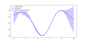
-
This reply was modified 3 months ago by Wolf.
-
This reply was modified 3 months ago by Wolf.
-
This reply was modified 3 months ago by
 yRocket.
-
This reply was modified 3 months ago by yRocket.
-
This reply was modified 3 months ago by yRocket.
-
This reply was modified 3 months ago by yRocket.
Calculating $k(x_{\ast}, x_{\ast})$ in Gaussian Processes
To understand how $k(x_{\ast}, x_{\ast})$ is calculated, you have to remember that the Kernel Function (or Covariance Function) is a mathematical rule that defines the relationship between any two points in your input space.
1. The Mathematical Definition
The term $k(x_{\ast}, x_{\ast})$ represents the prior variance at a specific test point $x_{\ast}$. In simpler terms, it answers the question: “Before we see any data, how much do we expect the function value at $x_{\ast}$ to vary?”
If we use the most common kernel, the Squared Exponential (RBF) Kernel, the formula is:
$$k(x, x’) = \sigma_f^2 \exp\left( -\frac{|x – x’|^2}{2\ell^2} \right)$$
When we evaluate this for the same point ($x = x_{\ast}$ and $x’ = x_{\ast}$):
1. The distance $|x_{\ast} – x_{\ast}|^2$ becomes 0.
2. The exponential term $\exp(0)$ becomes 1.
3. Therefore, $k(x_{\ast}, x_{\ast}) = \sigma_f^2$.
2. Physical Interpretation
In a standard GP setup, $k(x_{\ast}, x_{\ast})$ is usually a constant.
Component Interpretation Value It equals the vertical scale variance ($\sigma_f^2$) of your GP. Uncertainty It represents the “Maximum Uncertainty” the model has when it is infinitely far away from any training data. Diagonal Entry In the Joint Covariance Matrix, $k(x_{\ast}, x_{\ast})$ is the diagonal element for the test point.
3. How it fits into the Prediction
Recall the predictive variance formula we discussed earlier:
$$Var(f_{\ast}) = \underbrace{k(x_{\ast}, x_{\ast})}_{\text{Prior Uncertainty}} – \underbrace{K(x_{\ast}, X) K(X, X)^{-1} K(X, x_{\ast})}_{\text{Information Gain from Data}}$$
- Before Data: Your uncertainty is simply $k(x_{\ast}, x_{\ast})$.
- After Data: You subtract a positive value (the second term) based on how much the training data $X$ tells you about $x_{\ast}$.
- At a Training Point: If $x_{\ast}$ is exactly a training point, the second term cancels out the first, and $Var(f_{\ast})$ becomes 0 (assuming no noise).
4. Implementation Example
In Scikit-Learn or GPy, you don’t usually calculate this manually. The library computes the kernel matrix for you:
# Python # Assuming 'gp' is your trained model and 'x_star' is your test point kernel_function = gp.kernel_ # This computes the variance at x_star variance_at_x_star = kernel_function(x_star, x_star)-
This reply was modified 3 months ago by Wolf.
-
This reply was modified 3 months ago by Wolf.
-
This reply was modified 3 months ago by Wolf.
GP Prior vs. Posterior: The Bayesian View
In Gaussian Processes (GPs), the transition from Prior to Posterior represents the process of “learning” from data. Since a GP is a distribution over functions, this transition describes how our beliefs about which functions are possible change after we observe real data points.
1. The GP Prior (Before seeing data)
The Prior represents our initial assumptions about the function’s behavior (e.g., “it’s smooth,” “it’s periodic,” or “it stays near zero”).
- Definition: We assume the function values $f$ follow a Multivariate Normal Distribution with a mean of zero and a covariance defined by our kernel $K$.
- Visual: If you sample from a GP Prior, you get a “spaghetti” plot of many random, overlapping functions.
- Math: $$f(X) \sim \mathcal{N}(\mathbf{0}, K(X, X))$$
AI Learner Tip: In the Prior, the uncertainty (variance) is the same everywhere. The model has no reason to favor one path over another yet.
2. The GP Posterior (After seeing data)
The Posterior is the updated distribution after we have observed training data $\mathcal{D} = {(x_i, y_i)}$. We “force” the functions to pass through (or near) the observed data points.
- Mechanism: We use Bayes’ Rule:
$$P(f | \text{data}) = \frac{P(\text{data} | f) P(f)}{P(\text{data})}$$ - Result: The “spaghetti” of functions is pruned. Only the functions that are consistent with our observations remain.
- Visual: The functions now “pinch” together at the data points, where uncertainty becomes nearly zero.
3. Key Differences at a Glance
Feature GP Prior GP Posterior Data Involvement None (Assumptions only) Training data incorporated Mean ($\mu$) Usually $\mathbf{0}$ Shifted toward the data points Variance ($\sigma^2$) High and constant ($k(x, x)$) Low near data; High far from data Function Samples Wild and random Constrained to “fit” the observations
4. How the “Learning” Happens
When you move from Prior to Posterior, the GP performs a Joint Distribution calculation. It treats the training points $f$ and the new test point $f_{\ast}$ as part of one big Gaussian vector.
By applying the conditioning rule for Gaussians, the Posterior distribution for a new point $x_{\ast}$ becomes:
$$f_{\ast} | X, f, x_{\ast} \sim \mathcal{N}(\bar{f}_{\ast}, \text{cov}(f_{\ast}))$$
Where the mean $\bar{f}_{\ast}$ is a weighted sum of the training labels $y$, and the variance is reduced because the training data has provided information about the function’s local behavior.
Summary
- Prior: “I think the function is smooth, but I have no idea where it is.”
- Posterior: “I see the data at $x=1$ and $x=2$, so now I’m certain the function passes through those points, though I’m still guessing about $x=10$.”
-
AuthorPosts
- You must be logged in to reply to this topic.