
Modeling Thickness Variation in Semiconductor Thin-Film Processes — A Spatial Decomposition Approach to Machine Learning (ML)
Thickness uniformity in thin-film deposition determines downstream yield and device performance. Variation arises along two distinct axes — within a single wafer (Within-Wafer, WiW) and across wafers over time (Wafer-to-Wafer, W2W). These two axes have different physical origins and demand different diagnostic treatments. Mixing them into a single ML target forces the model to learn two unrelated physics simultaneously, hurting both.
This post presents an ML framework that incorporates Spatial Decomposition based on Zernike Polynomials (Zernike 1934; Noll 1976) into label engineering. It compresses 13-point wafer thickness measurements into 9 physically meaningful coefficients, which then serve as targets for a Two-Head ML architecture.
The framework is organized along three axes: Domain (facts), Design (technical choices), and Delivery (user value).
1. Domain
Domain defines the set of facts the model operates within: the environment, the data, and the mathematical tools available.
1.1 WiW / W2W Variation — Industrial Background
- W2W variation: temporal change in mean thickness per wafer. Driven by Run-to-Run drift, source/target depletion, recipe shifts.
- WiW variation: spatial thickness distribution within a single wafer. Driven by chamber hardware asymmetry, gas flow imbalance, temperature non-uniformity.
The two axes have different physical origins, so they require different diagnostic and control approaches. Treating them as a single ML target conflates two physics regimes and degrades both.
1.2 Measurement Setup — 13-Point Wafer Location Pattern
| Item | Value |
|---|---|
| Wafer size | 300 mm |
| Edge Exclusion (EE) | 5 mm |
| Number of points | 13 |
| Layout | Center 1 + Middle ring (r=75 mm, 4 cardinal) + Edge ring (r=145 mm, 8 directions) |
- Three radial levels (0 / 75 / 145 mm) — enables radial-order decomposition.
- Cardinal-aligned middle ring (0°/90°/180°/270°) — stabilizes astigmatism extraction.
- Edge ring at 8 directions — enables higher-order asymmetry (coma, trefoil) representation.
1.3 Dataset under Study
Output side (target source)
| Data | Form | Frequency |
|---|---|---|
| 13-point thickness measurements | 13 scalars per wafer (Å or nm) | per wafer or lot |
Input side (feature source)
| Data | Form | Use |
|---|---|---|
| Equipment sensor time-series — Fault Detection and Classification (FDC) | RF Power, Pressure, Gas Flow, Temperature, etc. | step-wise statistics for feature engineering |
| Process metadata | Recipe ID, Chamber ID, Timestamp | grouping variables, context |
| Preventive Maintenance (PM) / maintenance history | event log | baseline definition for drift analysis |
1.4 Zernike Polynomials — Mathematical Foundation
- Orthogonal basis functions defined on the unit disk (Zernike 1934).
- Each term is a function of normalized radius $\rho \in [0,1]$ and angle $\theta \in [0, 2\pi]$.
- Standard tool in optics and metrology for wavefront decomposition and surface form analysis (Born & Wolf 1999).
Decomposition formula:
where $T(\rho, \theta)$ is the thickness distribution, $Z_k$ is the $k$-th Zernike basis function, $a_k$ is the corresponding scalar coefficient, $\varepsilon$ is the residual, and $N$ is the number of terms used.
Physical meaning of low-order terms (Noll 1976 convention):
| Index | Name | Physical meaning |
|---|---|---|
| $Z_1$ | Piston | Mean thickness |
| $Z_2$ | Tilt X | Slope along X |
| $Z_3$ | Tilt Y | Slope along Y |
| $Z_4$ | Defocus | Bowl / Dome (center–edge contrast) |
| $Z_5$ | Astigmatism 45° | 45°/135° asymmetry |
| $Z_6$ | Astigmatism 0° | 0°/90° asymmetry |
| $Z_7$ | Coma Y | Y-direction asymmetric variation |
| $Z_8$ | Coma X | X-direction asymmetric variation |
| $Z_9$ | Trefoil | 3-fold pattern |
2. Design
Design covers the technical choices and optimization strategies built on top of the Domain — the realm of decisions and trade-offs.
2.1 Why Zernike Polynomials
| Candidate | Pros | Cons | Fit |
|---|---|---|---|
| Zernike Polynomials | Natural fit to circular domain, orthogonal, physically interpretable | Order must be capped for 13 points | ◎ |
| Polynomial ($x^n, y^n$) | Simple to implement | Non-orthogonal, unstable near circular edge | △ |
| Fourier series (polar) | Orthogonal in angle | Poor radial expressiveness | △ |
| Spline interpolation | Passes through measured points exactly | No physical meaning, noise-sensitive | ✗ |
| Principal Component Analysis (PCA) / Autoencoder | Data-driven compression | Not interpretable, requires large data | ✗ |
Five reasons Zernike wins for this problem: (1) the wafer is a disk and Zernike is defined on a disk — the coordinate systems align naturally; (2) orthogonality means each coefficient represents an independent pattern; (3) low-order terms map directly to known process drivers (tilt, bowl, astigmatism); (4) Zernike is the de-facto standard in optics and semiconductor metrology (Wang & Silva 1980); (5) compression from 13 points to 9 coefficients improves ML learning efficiency.
2.2 Spatial Decomposition Structure — W2W / WiW Separation
[Measurement space]            [Zernike space]

13 point values         ──►   9 coefficients
(T1, T2, ..., T13)             (a1, a2, ..., a9)

13-D                           9-D
(location-dependent)           (meaning-dependent)
W2W / WiW group definition:
| Group | Component | Count | Zernike terms | Meaning |
|---|---|---|---|---|
| W2W | Mean component | 1 | $Z_1$ (Piston) | Wafer-wide mean thickness |
| WiW | Shape components | 8 | $Z_2 \sim Z_9$ | Spatial variation (tilt / bowl / astigmatism / coma / trefoil) |
Three reasons for separation:
- Higher ML accuracy — W2W and WiW are different physics; separating them lets each head focus on its own signal, improving accuracy and convergence speed.
- Equipment fingerprint generation — the 8-element WiW vector forms a unique chamber signature that enables matching and outlier detection.
- Continuous thickness inference — 13 measurements reconstruct the full wafer thickness as a continuous function, allowing inference at unmeasured locations.
Fitting in matrix form:
where $T \in \mathbb{R}^{13 \times 1}$ is the measurement vector, $A \in \mathbb{R}^{13 \times 9}$ is the Zernike basis matrix, $a \in \mathbb{R}^{9 \times 1}$ is the coefficient vector to be estimated, and $\varepsilon \in \mathbb{R}^{13 \times 1}$ is the residual. Standard solution is Least Squares (LSQ); for noise robustness, Ridge Regression (Hoerl & Kennard 1970) is recommended. Detailed derivations appear in Appendices E and F.
With 13 measurements and 9 unknowns, the residual carries 4 degrees of freedom — sufficient for stable fitting and residual diagnostics. Higher-order terms ($Z_{10}$ and above) are under-determined and flow into the residual instead.
2.3 Model Architecture — Two-Head Design
                          ┌─► W2W Head ─► a1   (mean, 1 output)
Sensor data X ─► [Model] ─┤
                          └─► WiW Head ─► a2..a9 (shape, 8 outputs)
                                            │
                                            ▼
                                    Equipment fingerprint
- Input: feature vector X derived from sensor time-series.
- Output: 9 coefficients (1 W2W + 8 WiW).
- Reconstruction: 9 coefficients combined with Zernike basis yield $\hat{T}(\rho, \theta)$ at any location.
Two-Head benefits: separates loss between very different output scales (W2W large, WiW small); allows feature subset specialization per head since the driving factors differ; enables independent monitoring and retraining per head in operation.
2.4 Recommended Algorithms per Head
| Head / Group | 1st choice | 2nd choice | Rationale |
|---|---|---|---|
| W2W Head ($Z_1$) | Ridge Regression | XGBoost (shallow) | Strongly linear, interpretability priority, stable on small data |
| WiW low-order ($Z_2 \sim Z_4$) | LightGBM / XGBoost | Random Forest | Mild non-linearity, multivariate interactions |
| WiW high-order ($Z_5 \sim Z_9$) | XGBoost (heavy regularization) | 1D-CNN, Stacking | Small signal, noise robustness needed |
With sufficient data (> 5,000 wafers), a Multi-task Learning structure with a shared backbone and group-specific heads is effective.
2.5 Drift Tracking — Spatial × Temporal
Spatial decomposition compresses one wafer’s spatial pattern into 9 coefficients; temporal drift is then tracked on the time-series of those coefficients using Statistical Process Control (SPC) charts, Exponentially Weighted Moving Average (EWMA), or Cumulative Sum (CUSUM) — see Montgomery (2013).
[Spatial: Zernike]                   [Temporal: SPC / time-series]

T(ρ,θ; t)  →  (a1(t), ..., a9(t))  →  EWMA / CUSUM / ARIMA
(one wafer)    (coefficient series)    (drift detection)
- Spatial drift: captured by Zernike coefficients (e.g., gradual rise in $a_4$ = bowl deepening).
- Temporal drift: tracked on the 9 coefficient time-series using SPC, EWMA, or CUSUM.
- Non-Zernike patterns: point defects and local hot-spots are caught by residual monitoring instead.
2.6 Residual Interpretation and Use
The 13-D measurement decomposes into a 9-D Zernike fit plus a residual carrying 4 Degrees of Freedom (DOF):
13-D measurement
   │
   ├── 9-D (Zernike fit)  ──► ML training target
   │
   └── Residual (DOF 4)   ──► diagnostic information
| Residual component | Origin | Use |
|---|---|---|
| High-order spatial pattern | Process systematic missed by 9 terms | Signals model capacity insufficiency → consider order extension |
| Measurement system bias | Sensor calibration issue | Per-point reliability check |
| Local defect | Particle, scratch, etc. | Anomaly detection |
| Random noise | Measurement repeatability limit | Noise-floor estimation |
Two-layer monitoring strategy: Layer 1 (Zernike coefficients) tracks “expected variation” — drift detection, run-to-run control. Layer 2 (residual statistics) catches “unexpected anomalies” — alarm triggers, defect inspection.
2.7 Dimensionality Reduction Strategy
| Method | Characteristic | When to apply |
|---|---|---|
| Variance filter | Drop coefficients with low variability | After initial baseline analysis |
| Domain knowledge | Pick dominant terms per process type — Chemical Vapor Deposition (CVD) / Physical Vapor Deposition (PVD) / Atomic Layer Deposition (ALD) / Etch | When process priors are clear |
| Target correlation | Select terms most correlated with yield/quality | When outcome data is available |
| PCA on coefficients | Automatic compression (loses interpretability) | For ML input features only |
| Sparse Regression (Least Absolute Shrinkage and Selection Operator, LASSO) | Auto-selection during ML training | Integrated learning step |
Recommendation: split coefficients into “Active” (used for learning) and “Passive” (monitored only) groups. Don’t discard — keep computing and watching all coefficients.
3. Delivery
Delivery defines what the user gains by adopting this framework — operational and business value, not technical structure.
3.1 Application — Four Outcomes by W2W / WiW Group
| # | Group | Outcome | How |
|---|---|---|---|
| 1 | W2W | Run-to-Run thickness control | Mean trend tracking |
| 2 | WiW | Early outlier-tool detection | Fingerprint deviation |
| 3 | WiW | Preventive Maintenance (PM) timing optimization | Fingerprint trend |
| 4 | WiW | Hardware root-cause diagnosis | Pattern-to-factor mapping |
3.2 W2W Outcome — Run-to-Run Thickness Control
How: mean trend tracking. The W2W head’s predicted mean thickness ($\hat{a}_1$) drives recipe correction for the next wafer or lot, minimizing per-lot deviation and absorbing source-depletion or recipe-drift effects before they hit spec.
3.3 WiW Outcomes
Early outlier-tool detection. Monitor distance from a normal-baseline fingerprint (e.g., Mahalanobis distance) over the 8-element WiW vector. Detects deviating tools before yield impact, maintains chamber-to-chamber matching, ensures fleet-level consistency.
PM timing optimization. Move from periodic PM to condition-based PM driven by fingerprint drift trends. Improves uptime and reduces maintenance cost simultaneously, avoiding both unnecessary PMs and delayed-PM excursions.
Hardware root-cause diagnosis. Each shape coefficient maps to specific hardware factors:
- Tilt → chuck levelness, gas inlet position
- Bowl → center-edge temperature delta, RF coupling
- Astigmatism → showerhead directionality, magnetic-field asymmetry
- Coma / Trefoil → pump location, 3-zone heater non-uniformity
Result: faster root-cause identification on excursions, better maintenance efficiency, standardized troubleshooting playbooks.
Appendix A. 13-Point JSON Coordinate Definition
{
  "wafer_size_mm": 300,
  "edge_exclusion_mm": 5,
  "pattern": "13-points",
  "points": [
    {"id": "P1",  "x":    0.0, "y":    0.0, "r":   0, "theta":   0, "zone": "Center"},
    {"id": "P2",  "x":   75.0, "y":    0.0, "r":  75, "theta":   0, "zone": "Mid_E"},
    {"id": "P3",  "x":    0.0, "y":   75.0, "r":  75, "theta":  90, "zone": "Mid_N"},
    {"id": "P4",  "x":  -75.0, "y":    0.0, "r":  75, "theta": 180, "zone": "Mid_W"},
    {"id": "P5",  "x":    0.0, "y":  -75.0, "r":  75, "theta": 270, "zone": "Mid_S"},
    {"id": "P6",  "x":  145.0, "y":    0.0, "r": 145, "theta":   0, "zone": "Edge_E"},
    {"id": "P7",  "x":  102.5, "y":  102.5, "r": 145, "theta":  45, "zone": "Edge_NE"},
    {"id": "P8",  "x":    0.0, "y":  145.0, "r": 145, "theta":  90, "zone": "Edge_N"},
    {"id": "P9",  "x": -102.5, "y":  102.5, "r": 145, "theta": 135, "zone": "Edge_NW"},
    {"id": "P10", "x": -145.0, "y":    0.0, "r": 145, "theta": 180, "zone": "Edge_W"},
    {"id": "P11", "x": -102.5, "y": -102.5, "r": 145, "theta": 225, "zone": "Edge_SW"},
    {"id": "P12", "x":    0.0, "y": -145.0, "r": 145, "theta": 270, "zone": "Edge_S"},
    {"id": "P13", "x":  102.5, "y": -102.5, "r": 145, "theta": 315, "zone": "Edge_SE"}
  ]
}Appendix B. 13-Point Wafer Location Map
                          N (+Y)
                           │
                    . . . P8 . . .
                .       (0,145)      .
            P9 .                      . P7
        (-102,102).                  .(102,102)
           .          P3 (0,75)         .
          .               │              .
         .                │               .
        .                 │                .
       .                  │                 .
      P10─────P4─────────P1─────────P2─────P6   ── E (+X)
    (-145,0)(-75,0)    (0,0)     (75,0) (145,0)
       .                  │                 .
        .                 │                .
         .                │               .
          .          P5 (0,-75)          .
           .              │             .
       P11 .                            . P13
       (-102,-102) .                . (102,-102)
                .       (0,-145)      .
                    . . . P12 . . .
                           │
                          S (-Y)
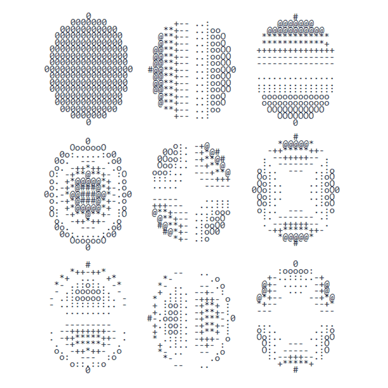
Appendix C. Visualization of Low-Order Zernike Terms
Each Zernike term is rendered as a 17×17 ASCII grid normalized to its own peak, so shape patterns are directly comparable across terms.
Shading legend (negative ← zero → positive):
   #   @   *   +   -   ' '   .   :   o   O   0
strong                                       strong
negative              zero                   positive
C.1 $Z_1$ — Piston (mean)
$(n=0, m=0)$ — wafer-wide constant. Captures the mean thickness; the W2W variation lives here.
        0
     0000000
   00000000000
  0000000000000
  0000000000000
 000000000000000
 000000000000000
 000000000000000
00000000000000000
 000000000000000
 000000000000000
 000000000000000
  0000000000000
  0000000000000
   00000000000
     0000000
        0
C.2 $Z_2$ — Tilt X
$(n=1, m=1)$ — linear slope along X. Diagnoses chuck levelness or asymmetric gas inlet position.
     +-- ..:
   **+-- ..:oo
  @**+-- ..:ooO
  @**+-- ..:ooO
 @@**+-- ..:ooOO
 @@**+-- ..:ooOO
 @@**+-- ..:ooOO
#@@**+-- ..:ooOO0
 @@**+-- ..:ooOO
 @@**+-- ..:ooOO
 @@**+-- ..:ooOO
  @**+-- ..:ooO
  @**+-- ..:ooO
   **+-- ..:oo
     +-- ..:
C.3 $Z_3$ — Tilt Y
$(n=1, m=-1)$ — linear slope along Y. Diagnoses front-back chuck levelness or top-bottom flow asymmetry.
        #
     @@@@@@@
   @@@@@@@@@@@
  *************
  ************+
 +++++++++++++++
 ---------------
 ---------------

 ...............
 ...............
 :::::::::::::::
  ooooooooooooo
  ooooooooooooo
   OOOOOOOOOOO
     OOOOOOO
        0
C.4 $Z_4$ — Defocus (Bowl / Dome)
$(n=2, m=0)$ — radially symmetric center-vs-edge contrast. Key diagnostic for center-edge temperature delta, RF coupling, and showerhead-to-wafer gap.
        0
     OoooooO
   0o:.....:o0
  0o.  ---  .o0
  o. -++*++- .o
 O: -+**@**+- :O
 o. +*@@@@@*+ .o
 o.-+*@###@*+-.o
0o.-*@@###@@*-.o0
 o.-+*@###@*+-.o
 o. +*@@@@@*+ .o
 O: -+**@**+- :O
  o. -++*++- .o
  0o.  ---  .o0
   0o:.....:o0
     OoooooO
        0
C.5 $Z_5$ — Astigmatism 45°
$(n=2, m=-2)$ — 4-fold asymmetry along diagonals. Diagnoses 45°/135°-direction flow asymmetry or magnetic-field bias.
     o:. -+@
   0Oo:. -+*@#
  0Ooo:. -+**@#
  Ooo:.. --+**@
 ooo:..  ---+**@
 :::...   ---+++
 .....     -----

 -----     .....
 +++---   ...:::
 @**+--- ...:ooo
  @**+-- ..:ooO
  #@**+- .:ooO0
   #@*+- .:oO0
     *+- .:o
C.6 $Z_6$ — Astigmatism 0°
$(n=2, m=2)$ — 4-fold asymmetry along horizontal/vertical. Diagnoses showerhead directionality and 0°/90° pump-position effects.
        #
     *@@@@@*
   -++*****++-
  . --+++++-- .
  :. ------- .:
 o:..  ---  ..:o
 Oo:.       .:oO
 Oo:..     ..:oO
0Oo:..     ..:oO0
 Oo:..     ..:oO
 Oo:.       .:oO
 o:..  ---  ..:o
  :. ------- .:
  . --+++++-- .
   -++*****++-
     *@@@@@*
        #
C.7 $Z_7$ — Coma Y
$(n=3, m=-1)$ — Y-direction asymmetric tilt with stronger curvature on one side. Diagnoses asymmetric Y flow and pump-position bias.
        #
     *++-++*
   *+  ...  +*
  *- .::o::. -*
  - .:ooooo:. -
 - .::ooooo::. -
 - ..:::::::.. -
    .........

    ---------
 . --+++++++-- .
 . -++*****++- .
  . -+*****+- .
  o. -++*++- .o
   o:  ---  :o
     o::.::o
        0
C.8 $Z_8$ — Coma X
$(n=3, m=1)$ — X-direction asymmetric tilt. Diagnoses asymmetric X gas inlet/outlet or one-sided chamber hardware bias.
     --   ..
   *-       .o
  *- ..   -- .o
  + .:.. --+- :
 * .:::. -+++- o
 + :oo:. -+**+ :
 +.:oo:. -+**+-:
#-.ooo:. -+***-.0
 +.:oo:. -+**+-:
 + :oo:. -+**+ :
 * .:::. -+++- o
  + .:.. --+- :
  *- ..   -- .o
   *-       .o
     --   ..
C.9 $Z_9$ — Trefoil (3-fold)
$(n=3, m=-3)$ — 3-fold pattern repeating every 120°. Marks 3-zone heater non-uniformity or 3-fold chamber hardware effects (3-leg lift pins, 3-port gas).
        0
     :ooooo:
   +-..:::..-+
  @+- ..... -+@
  @+-  ...  -+@
 @*+--     --+*@
 *+--       --+*
 ---         ---

 ...         ...
 o:..       ..:o
 Oo:..     ..:oO
  O:.  ---  .:O
  O:. ----- .:O
   :.--+++--.:
     +*****+
        #
C.10 Drift Diagnostic Guide
| Coefficient that suddenly grows | Hypothesized cause |
|---|---|
| $a_1$ (Piston) | Source depletion, deposition time/power shift |
| $a_2, a_3$ (Tilt) | Chuck levelness change, gas inlet position |
| $a_4$ (Defocus) | Center-edge temperature change, RF coupling, showerhead distance |
| $a_5, a_6$ (Astigmatism) | Showerhead directionality, magnetic-field asymmetry, pump position |
| $a_7, a_8$ (Coma) | Asymmetric gas flow, one-sided hardware bias |
| $a_9$ (Trefoil) | 3-zone heater or 3-fold hardware issues |
Appendix D. Why 13 Measurements Map to 9 Coefficients
For a linear measurement model $T = A \cdot a + \varepsilon$ with $m$ measurements and $N$ basis terms, three regimes exist:
| Condition | Name | Result |
|---|---|---|
| $N > m$ | Under-determined | Infinitely many solutions — no unique answer |
| $N = m$ | Exactly-determined | Residual = 0 but noise also fitted (overfitting) |
| $N < m$ | Over-determined | Residual-minimizing LSQ solution exists — recommended |
For 13 points, the choice of $N$ is constrained:
| $N$ | Patterns expressible | DOF | Verdict |
|---|---|---|---|
| 4 | Piston, Tilt X/Y, Defocus | 9 | Insufficient (no asymmetry) |
| 6 | + Astigmatism 0°/45° | 7 | Acceptable |
| 9 | + Coma X/Y, Trefoil | 4 | Recommended balance |
| 11 | + Spherical, Quadrafoil | 2 | DOF too low |
| 13 | + further terms | 0 | No residual monitoring possible |
DOF of 4 means the residual $\varepsilon$ moves freely in a 4-dimensional subspace, providing the information channel for residual diagnostics (Section 2.6). The 13 → 9 mapping is therefore not an arbitrary choice but the simultaneous optimum of three constraints: over-determined system, sufficient expressiveness, and residual-monitoring DOF.
Appendix E. Zernike basis matrix A
The model: $T = A \cdot a + e$
The Zernike decomposition writes a measured wavefront $T$ as a linear combination of Zernike basis functions plus measurement noise:
$$T = A \cdot a + e$$
This appendix walks through what each piece of the equation means and what makes $A$ — the Zernike basis matrix — useful.
Symbols
The pieces of the model carry the following meaning:
| Symbol | Meaning |
|---|---|
| $Z_j(\rho, \theta)$ | The $j$-th Zernike basis function on the unit disk |
| $(\rho_i, \theta_i)$ | Polar coordinates of the $i$-th measurement point |
| $a_j$ | Coefficient (weight) of $Z_j$ — the unknown to fit |
| $T_i$ | Measured value at the $i$-th point (e.g. wafer thickness) |
| $e_i$ | Measurement noise at the $i$-th point |
$Z_j$ is one element of a sequence of fixed shapes defined on the unit disk (the disk of radius $1$). Just as a Fourier series uses sines and cosines as a basis, a Zernike expansion uses $Z_1, Z_2, Z_3, \ldots$ as its basis. The Noll convention numbers the basis functions starting from $j = 1$.
| $j$ | Shape of $Z_j$ | Optical name |
|---|---|---|
| 1 | constant (flat) | Piston |
| 2 | tilt along $x$ | Tilt X |
| 3 | tilt along $y$ | Tilt Y |
| 4 | bowl (center vs. edge) | Defocus |
| $\ldots$ | $\ldots$ | $\ldots$ |
For the $i$-th measurement point, $\rho_i$ is the radius from the disk center (normalized so that the edge sits at $\rho = 1$) and $\theta_i$ is the angle from the positive $x$-axis (in radians).
Per-point equation
Written out for one point $i$, the model becomes:
$$T_i = a_1 Z_1(\rho_i, \theta_i) + a_2 Z_2(\rho_i, \theta_i) + \ldots + a_N Z_N(\rho_i, \theta_i) + e_i$$
Each measurement is decomposed into a weighted sum of $N$ predefined shapes; the unknowns are the weights $a_j$. Stacking the $m$ such per-point equations gives the matrix form $T = A \cdot a + e$.
Structure of $A$ ($m \times N$)
The entries of $A$ are Zernike-basis evaluations at the measurement points:
$$A[i, j] = Z_j(\rho_i, \theta_i)$$
That is, $A[i, j]$ is “the value of the $j$-th basis at the $i$-th measurement point”. $A$ has $m$ rows (one per measurement point) and $N$ columns (one per Zernike basis function):
            j=1     j=2     j=3    ...   j=N
        ┌─────────────────────────────────────┐
i=1     │  Z_1    Z_2    Z_3    ...    Z_N    │ ← all basis values at point 1
i=2     │  Z_1    Z_2    Z_3    ...    Z_N    │ ← all basis values at point 2
...     │   …      …      …             …     │
i=m     │  Z_1    Z_2    Z_3    ...    Z_N    │ ← all basis values at point m
        └─────────────────────────────────────┘
          ↑
        column 1 = Z_1 evaluated at every measurement point
Row and column meaning
The rows and columns of $A$ have very different meanings, and both are useful:
- Column $j$: the values of one fixed basis function $Z_j$ sampled at all $m$ measurement points — $Z_j$’s sampling pattern at the measurement points (the $j$-th column vector of $A$). It is a snapshot of the continuous function $Z_j$ “photographed” at the chosen $m$ points.
- Row $i$: the values of all $N$ basis functions evaluated at one measurement point — the coefficients on the right-hand side of the expansion equation (writing the wavefront as a sum of basis functions) at that point.
Here expansion means writing a function as a sum of basis functions. The Fourier series, which expands a function as a sum of sines and cosines, is the textbook example. In Zernike land we expand the wavefront $T(\rho, \theta)$ as a sum of $Z_j$.
Noll normalization
The Noll convention scales each $Z_j$ so that all coefficients $a_j$ are directly comparable. After normalization, on the unit disk:
$$\iint_{\text{disk}} Z_j(\rho, \theta)^2 \, dA = \pi \quad \text{for every } j \quad\text{(unit norm)}$$
$$\iint_{\text{disk}} Z_j \, Z_k \, dA = 0 \quad \text{for } j \neq k \quad\text{(orthogonality)}$$
The scaling constants depend on the $(n, m)$ pair (radial order $n$, azimuthal frequency $m$) that each $j$ corresponds to:
- For $m = 0$ terms (purely radial: Piston, Defocus, …): multiply by $\sqrt{n+1}$.
- For $m \neq 0$ terms (with $\cos$ or $\sin$: Tilt, Astigmatism, …): multiply by $\sqrt{2(n+1)}$.
The $j \rightarrow (n, m)$ conversion follows Noll’s 1976 algorithm. The benefit of normalization: $a_j^2$ is exactly “$j$’s contribution to the wavefront RMS”, so absolute coefficient values can be compared at a glance.
$A^{\!\top}\!A \approx m \cdot I$ — sampling density and regression stability
The least-squares solution is $\hat{a} = (A^{\!\top}\!A)^{-1} A^{\!\top}\, T$, so the structure of $A^{\!\top}\!A$ controls the conditioning of the fit. Its $(j, k)$ entry is the inner product of column $j$ and column $k$ of $A$:
$$(A^{\!\top}\!A)_{jk} = \sum_{i=1}^{m} Z_j(\rho_i, \theta_i)\, Z_k(\rho_i, \theta_i)$$
Dense sampling ($m \rightarrow \infty$, with the points uniformly covering the disk): the discrete sum tends to the integral average:
$$\frac{1}{m} \sum_{i=1}^{m} Z_j(\rho_i, \theta_i)\, Z_k(\rho_i, \theta_i) \;\approx\; \frac{1}{\pi} \iint_{\text{disk}} Z_j Z_k \, dA \;=\; \delta_{jk}$$
hence $A^{\!\top}\!A \approx m \cdot I$ — a diagonal matrix with all diagonal entries equal to $m$. In this regime:
- $(A^{\!\top}\!A)^{-1} \approx I/m$ — the inverse is essentially “multiply by $1/m$”. Numerically very stable.
- $\hat{a}_j \approx \frac{1}{m} \sum_i Z_j(\rho_i, \theta_i)\, T_i$ — each coefficient is just a $Z_j$-weighted average of the measurements.
- Condition number $\approx 1$ — measurement noise propagates to the coefficients with virtually no amplification.
Sparse sampling (e.g. the $m = 13$ measurement points used in this project): the integral approximation breaks. $A^{\!\top}\!A$ is no longer diagonal; it is a general $N \times N$ matrix with non-zero off-diagonal entries, and its condition number grows. With $m = 13 \geq N = 9$ the fit is still solvable, but if the condition number becomes too large, ridge regression (adding $\lambda I$ to $A^{\!\top}\!A$) is a standard way to stabilize the solve.
Appendix F. Least Squares Normal-Equation Derivation
Find the coefficients that minimize squared residual:
Expanding the objective $J(a) = \| T – A \cdot a \|^2$:
Setting $\partial J / \partial a = 0$:
This is the normal equation. When $A^\top A$ is invertible (i.e., $A$ has full column rank), the solution is:
Geometrically, $\hat{a}$ is the orthogonal projection of $T$ onto the column space of $A$, so the residual $\varepsilon = T – A \cdot \hat{a}$ satisfies $A^\top \varepsilon = 0$. The Hessian $2 A^\top A$ is positive semi-definite, so this is a global minimum.
For 13-point fitting, $A$ must have full column rank — the cardinal-aligned 13-point pattern satisfies this for $N=9$. If $A^\top A$ is ill-conditioned, use SVD-based pseudo-inverse or Ridge Regression (Appendix G).
Appendix G. Ridge Regression Derivation (Tikhonov Regularization)
Pure LSQ becomes unstable when $A^\top A$ is ill-conditioned or measurement noise is large. Hoerl & Kennard (1970) addressed this by adding an L2 penalty to the objective:
where $\lambda \geq 0$ is the regularization strength. With $\lambda = 0$ this reduces to LSQ; as $\lambda \to \infty$, $a \to 0$. Expanding:
Setting the gradient to zero:
Why this is always invertible: if $A^\top A$ is positive semi-definite, then for any $\lambda > 0$, $A^\top A + \lambda I$ is strictly positive-definite — guaranteeing a unique solution even when LSQ fails.
| Aspect | LSQ | Ridge |
|---|---|---|
| Singular $A^\top A$ | No solution | Solution exists |
| Noise sensitivity | High | Low |
| High-order coefficient stability | Unstable | Stable |
| Bias | None | Mild bias introduced |
| 13-point recommendation | Only when noise is very small | Recommended in general |
To choose $\lambda$ for 13-point fitting: collect coefficient distributions from many normal wafers via LSQ, sweep $\lambda \in \{0.001, 0.01, 0.1, 1.0, 10.0\}$, run Leave-One-Out Cross-Validation (LOOCV) by holding out one of the 13 measurements, pick the $\lambda$ minimizing average prediction error, and re-evaluate periodically (every few months).
References
- Born, M., & Wolf, E. (1999). Principles of Optics (7th ed.). Cambridge University Press.
- Hoerl, A. E., & Kennard, R. W. (1970). Ridge regression: Biased estimation for nonorthogonal problems. Technometrics, 12(1), 55–67.
- Montgomery, D. C. (2013). Introduction to Statistical Quality Control (7th ed.). Wiley.
- Noll, R. J. (1976). Zernike polynomials and atmospheric turbulence. Journal of the Optical Society of America, 66(3), 207–211.
- Wang, J. Y., & Silva, D. E. (1980). Wavefront interpretation with Zernike polynomials. Applied Optics, 19(9), 1510–1518.
- Zernike, F. (1934). Beugungstheorie des Schneidenverfahrens und seiner verbesserten Form, der Phasenkontrastmethode. Physica, 1(7–12), 689–704.