
The Impact of Variance Components on the Coefficient of Determination ($R^2$)
1. Executive Summary
The Coefficient of Determination, denoted as $R^2$, is one of the most widely used metrics for assessing the goodness-of-fit in linear regression models. However, its interpretation is often fraught with misunderstanding, particularly regarding how it fluctuates not just with the “correctness” of a model, but with the underlying distribution of the data. This report explores the mathematical and conceptual reasons why changes in variance—specifically residual variance ($\sigma^2_{\epsilon}$) and predictor variance ($\sigma^2_{x}$)—exert a profound influence on $R^2$. By analyzing the ratio of variances, we demonstrate that $R^2$ is a relative measure of power rather than an absolute measure of model accuracy.
2. Mathematical Definition of $R^2$
To understand why variance dictates the behavior of $R^2$, we must first define it through the lens of Analysis of Variance (ANOVA). In a standard linear model $Y = \beta_0 + \beta_1 X + \epsilon$, the total variation in the dependent variable $Y$ can be partitioned into two distinct components:
- Explained Variation (SS_{reg}): The variation accounted for by the relationship between $X$ and $Y$.
- Unexplained Variation (SS_{res}): The variation resulting from the residuals or “noise” ($\epsilon$).
The fundamental identity is:
$$SS_{tot} = SS_{reg} + SS_{res}$$
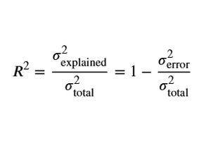
From this, $R^2$ is defined as the proportion of the total variance in $Y$ that is explained by $X$:
$$R^2 = \frac{SS_{reg}}{SS_{tot}} = 1 – \frac{SS_{res}}{SS_{tot}}$$
Where:
- $SS_{res}$ (Residual Sum of Squares): $\sum (y_i – \hat{y}_i)^2$
- $SS_{tot}$ (Total Sum of Squares): $\sum (y_i – \bar{y})^2$
3. The Impact of Increased Error Variance (Noise)
The first scenario involves an increase in the variance of the residuals ($\sigma^2_{\epsilon}$), assuming the true relationship ($\beta_1$) and the range of $X$ remain constant.
3.1 The Mathematical Mechanism
As the noise in the data increases, each observed value $y_i$ deviates further from the regression line $\hat{y}i$. This directly inflates the $SS{res}$ term. In the formula $R^2 = 1 – \frac{SS_{res}}{SS_{tot}}$, as the numerator of the fraction increases, the entire fraction $\frac{SS_{res}}{SS_{tot}}$ grows larger. Consequently, when this larger value is subtracted from 1, the resulting $R^2$ decreases.
3.2 Conceptual Interpretation: The Signal-to-Noise Ratio
In the context of information theory and machine learning, we view the relationship between $X$ and $Y$ as the Signal and the residuals as the Noise. When the error variance increases, the noise overwhelms the signal. Even if the underlying model is “correct” (i.e., you have identified the true $\beta_1$), the predictive power is diluted.
Key Phrase: “Increased noise or residual variance diminishes the model’s explanatory power, leading to a lower $R^2$.”
This illustrates that a low $R^2$ does not necessarily mean the model is “wrong”; it may simply mean the environment is inherently noisy, making the dependent variable difficult to predict with high precision.
4. The Impact of Increased Predictor Variance (Range of X)
A more counterintuitive phenomenon occurs when we change the variance of the independent variable $X$. If we expand the range of $X$ values (thereby increasing $\sigma^2_{x}$), the $R^2$ typically increases, even if the error variance $\sigma^2_{\epsilon}$ remains exactly the same.
4.1 The Expansion of the Denominator
In a simple linear regression, the explained variance can be expressed as:
$$SS_{reg} = \beta_1^2 \cdot \sum (x_i – \bar{x})^2$$
When the variance of $X$ increases, $\sum (x_i – \bar{x})^2$ increases. This causes $SS_{reg}$ to grow. Since $SS_{tot} = SS_{reg} + SS_{res}$, and $SS_{res}$ is assumed constant, the denominator $SS_{tot}$ grows primarily because the “explained” part is growing.
In the fraction $\frac{SS_{res}}{SS_{tot}}$, the denominator is getting larger while the numerator stays the same. This makes the fraction smaller, and $1 – (\text{smaller number})$ results in a higher $R^2$.
4.2 The Strength of the Trend
When we measure $X$ over a wider range, the overall “trend” or slope becomes more dominant relative to the local fluctuations (noise). The model captures a larger portion of the total spread of $Y$ because that spread is now driven more by the change in $X$ than by the random error.
Key Phrase: “A wider range or higher variance in the independent variable often inflates the $R^2$, as the model captures a larger portion of the overall trend.”
5. Summary Table: Variance vs. $R^2$
The following table summarizes the relationship between variance components and the resulting coefficient of determination.
| Scenario | Effect on $R^2$ | Statistical Reason |
|---|---|---|
| Higher Residual Variance ($\sigma^2_{\epsilon}$) | Decreases | The “unexplained” portion ($SS_{res}$) of the data becomes a larger fraction of the total. |
| Higher Predictor Variance ($\sigma^2_{x}$) | Increases | The “explained” portion ($SS_{reg}$) grows, making the noise relatively less significant. |
| Lower Total Variance ($SS_{tot}$) | Decreases | When the total spread of $Y$ is small, even minor errors lead to a low $R^2$. |
6. Practical Implications for AI/ML Models
In machine learning, relying solely on $R^2$ can be misleading due to these variance dependencies.
- Model Comparison: One cannot easily compare the $R^2$ of a model trained on a narrow dataset with one trained on a diverse, wide-ranging dataset. The latter will likely have a higher $R^2$ simply due to the variance in $X$.
- Overfitting Risks: High variance in $X$ can sometimes mask poor model performance in specific sub-regions of the data.
- Feature Selection: When adding features, we are essentially trying to increase the explained variance ($SS_{reg}$) to reduce the relative weight of the residuals.
7. Conclusion: $R^2$ as a Relative Metric
The reason why changes in variance affect $R^2$ is that $R^2$ is a ratio. It does not measure the absolute magnitude of the error (like MSE or MAE), but rather the error relative to the total spread of the data.
- If the Unexplained Variance increases, the ratio of “error to total” rises, and $R^2$ falls.
- If the Explained Variance increases (via a wider range of $X$), the ratio of “error to total” falls, and $R^2$ rises.
Understanding this dynamic is crucial for any data analyst or machine learning engineer. It prevents the common pitfall of dismissing a model with a low $R^2$ in a high-noise environment, or over-trusting a model with a high $R^2$ derived from an artificially wide range of independent variables.
8. Key Terminology Reference
- Coefficient of Determination ($R^2$): 결정계수. The proportion of variance in the dependent variable that is predictable from the independent variable.
- Explanatory Power: 설명력. The capacity of a model to represent the underlying patterns in the data.
- Residual/Error Variance: 잔차/오차 분산. The variance of the differences between observed and predicted values.
- Signal-to-Noise Ratio (SNR): 신호 대 잡음비. A measure that compares the level of a desired signal to the level of background noise.
9. $R^2$ Variation with Sample Distributions Placed Along the 1‑to‑1 Line
