
One-Hot Encoding Pitfalls and Countermeasures
1. What is One-Hot Encoding?
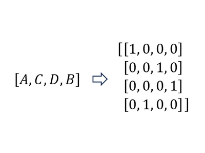
One-hot encoding is the most fundamental technique for converting categorical variables into numerical vectors that machine learning models can process. Given N unique categories, each category is represented as an N-dimensional vector with a 1 at the position corresponding to that category and 0 elsewhere.
Example: ['Seoul', 'Busan', 'Daegu'] → Seoul = [1,0,0], Busan = [0,1,0], Daegu = [0,0,1]
The advantages are that it imposes no arbitrary ordering between categories and guarantees mutual independence between them. It remains the default starting point for low-cardinality categorical variables.
2. Limitations of One-Hot Encoding
One-hot encoding suffers from two fundamentally different but equally important weaknesses: it explodes in dimensionality, and it destroys any natural ordering that may exist among categories. Both must be understood to choose the right alternative.
2.1 The Essence of the Curse of Dimensionality
First named by Richard Bellman in 1961, the curse of dimensionality refers to the exponential problems that arise as data dimensionality grows. In the context of one-hot encoding, the following effects become particularly severe:
(1) Explosion of Sparsity
Encoding a feature with 10,000 unique values (e.g., user_id, product_id) produces a 10,000-dimensional vector in which only 1 entry is 1 and 9,999 are 0. Memory usage explodes as O(N×D), and information density collapses to 1/D.
(2) Distance Concentration
In high-dimensional space, all pairwise Euclidean distances become nearly equal. Mathematically, as dimensionality d grows, the ratio of maximum to minimum distance converges to 1: lim(d→∞) (max_dist - min_dist) / min_dist → 0. This neutralizes distance-based algorithms like KNN and K-means.
(3) Sample Complexity Explosion
The number of samples needed to “fill” the input space grows exponentially with dimensionality. If 10 samples per dimension suffice, 100 dimensions would require 10^100 samples.
(4) Overfitting Risk
Rare categories appear as one-hot dimensions that are almost always 0, making them extremely susceptible to overfitting.
(5) Loss of Semantic Relationships
“Seoul” and “Busan” share the semantic concept of “city,” but in one-hot encoding they are perfectly orthogonal vectors with cosine similarity of 0. No relational structure can be learned.
(6) Tree-Model Splitting Bias
In decision-tree algorithms, sparse one-hot features almost always create “0 vs 1” splits. Information gain becomes distorted, and these features are systematically disadvantaged compared to continuous features.
2.2 Loss of Sequence and Ordinal Structure
Many real-world categorical variables carry an intrinsic order — education level (elementary < middle < high < bachelor < master < PhD), severity grade (mild < moderate < severe < critical), Likert-scale survey responses (strongly disagree → strongly agree), age brackets, customer tiers (bronze < silver < gold < platinum), and more. One-hot encoding erases this ordering completely, treating every level as equidistant and unrelated. This is a structural limitation that is independent of the curse of dimensionality, and in many domains it is the more damaging defect.
(1) Equidistance Assumption
For one-hot vectors, every pair of categories has the same Euclidean distance of √2 and the same cosine similarity of 0. The model receives no signal that “bachelor” is closer to “master” than to “elementary.” Any ordinal information must be re-discovered by the model from the target signal alone, which requires far more data and is often unreliable for rare levels.
(2) Loss of Monotonicity
In domains like credit scoring, healthcare risk, and pricing, regulators and stakeholders often require monotonic behavior — for example, “higher education should not lower predicted income.” With one-hot encoding, levels are independent, so monotonicity cannot be expressed or enforced. Tools like monotone_constraints in GBDT libraries become inapplicable because the constraint requires a single ordered numeric feature.
(3) Inability to Interpolate or Extrapolate
If training data lacks the “gold” tier but contains “silver” and “platinum,” a model with one-hot features has no basis for predicting “gold” sensibly. An ordinal or embedding-based representation can interpolate between neighboring levels; one-hot cannot.
(4) Loss of Sequential / Temporal Pattern
For categorical features that represent stages in a sequence — purchase funnel steps, disease progression stages, weekday/month, or pipeline stages — one-hot encoding loses adjacency. “Monday” and “Tuesday” are no closer than “Monday” and “Saturday.” Neural sequence models built on top of one-hot inputs must spend capacity learning trivial adjacency facts.
(5) Increased Sample Requirement for Ordinal Tasks
Because no order prior is provided, every level effectively becomes its own free parameter. Rare ordinal levels require many examples to be learned correctly, whereas an ordinal encoding would inherit information from neighboring levels for free.
(6) Statistical Interpretability Loss
In regression analysis, one-hot dummy variables produce one coefficient per level — the analyst cannot directly read off “the linear trend of severity on outcome.” Polynomial contrast or backward-difference coding preserve this trend explicitly.
Why This Matters in Practice
The two limitations compound. A high-cardinality ordinal feature (e.g., income decile across 100 bands, or 50 age buckets) suffers both the curse of dimensionality and the loss of ordering. Choosing the right encoding — ordinal integer + monotonic constraint, thermometer encoding, ordinal entity embedding, CORAL/CORN, or order embeddings — directly attacks both problems at once. This is why the practical guide in Section 8 explicitly distinguishes “order present” cases from “no order” cases.
3. Classical Solutions
These are deterministic or lightly-learned encodings that have served as the backbone of categorical handling for decades.
Label / Ordinal Encoding — Map categories directly to integers. Only valid when a meaningful order exists.
Frequency Encoding — Replace each category with its occurrence count. Simple, but cannot distinguish categories with equal frequency.
Target (Mean) Encoding — Replace categories with the mean of the target variable. Carries leakage risk, requiring K-fold splitting, smoothing, or noise injection.
Hash Encoding (Feature Hashing) — Map categories to a fixed-size bucket via a hash function. Memory-efficient but suffers collisions. Used in Vowpal Wabbit.
Binary / BaseN Encoding — Encode categories as binary (or base-N) numbers, reducing dimensionality to log₂(N).
Leave-One-Out Encoding, WOE (Weight of Evidence) — Common variants in finance and credit scoring.
Ordinal-Aware Classical Encodings — For variables with intrinsic order (education level, severity, Likert scale):
- Thermometer / Unary Encoding: Encode level k as k ones followed by zeros, e.g., level 2 of 3 → [1,1,0]. Naturally encodes partial order; underpins later ordinal deep learning methods (CORAL, CORN).
- Polynomial Contrast Coding: Decomposes ordinal effects into linear, quadratic, and cubic trends.
- Helmert / Reverse-Helmert Coding: Compares each level to the mean of subsequent (or preceding) levels.
- Backward Difference Coding: Encodes only differences between adjacent levels.
- Sum (Deviation) Coding: Compares each level to the grand mean.
These contrast-coding schemes remain standard in medicine, social sciences, and any setting where regression-coefficient interpretability matters.
4. Deep Learning-based Entity Embedding
Although introduced after the strictly statistical era, entity embeddings are now considered a classical, standard tool in any deep-learning workflow. The 2016 paper by Guo & Berkhahn — “Entity Embeddings of Categorical Variables” — proved their value in the Kaggle Rossmann Store Sales competition (3rd place). A decade later, they are the default choice for medium- and high-cardinality features.
Core Idea
Each category is mapped to a learnable, low-dimensional dense vector via an embedding layer placed at the front of the network. This is essentially the same mechanism as Word2Vec, applied to tabular data.
- Dimensionality: N → d, typically d ≈ min(50, (N+1)//2)
- Semantically similar categories cluster naturally in embedding space
- End-to-end gradient-based training optimizes the embedding for the downstream task
Ordinal-Preserving Embedding Variants
For categorical variables with intrinsic order, several extensions exist:
- Order Embeddings (Vendrov et al., ICLR 2016): Encode partial order via coordinate-wise inequality in the embedding space.
- Poincaré / Hyperbolic Embeddings (Nickel & Kiela, 2017): Embed hierarchical and ordered structures in hyperbolic space, where tree depth maps naturally to distance.
- Monotonic Embedding Networks: Use UMNN or Deep Lattice Networks to enforce monotonic structure.
- Order-Preserving Contrastive Learning (2023+): Triplet objectives enforce that
x < y < zimpliesd(x,y) < d(x,z).
The fastai TabularLearner and PyTorch’s nn.Embedding standardized this approach across the industry.
PyTorch Implementation Example
import torch
import torch.nn as nn
import pandas as pd

# Sample data with mixed categorical and numerical features
df = pd.DataFrame({
    'city':    ['Seoul', 'Busan', 'Daegu', 'Seoul', 'Incheon', 'Busan'],
    'product': ['A', 'B', 'A', 'C', 'B', 'A'],
    'price':   [100, 200, 150, 300, 250, 180],
    'target':  [1, 0, 1, 0, 1, 0],
})

# Map each category to an integer index
city_to_idx    = {c: i for i, c in enumerate(df['city'].unique())}
product_to_idx = {p: i for i, p in enumerate(df['product'].unique())}

df['city_idx']    = df['city'].map(city_to_idx)
df['product_idx'] = df['product'].map(product_to_idx)

n_cities, n_products = len(city_to_idx), len(product_to_idx)

# Rule of thumb: embedding dim = min(50, (cardinality + 1) // 2)
city_dim    = min(50, (n_cities + 1) // 2)
product_dim = min(50, (n_products + 1) // 2)

class EntityEmbeddingNet(nn.Module):
    def __init__(self):
        super().__init__()
        # Learnable lookup tables — replace one-hot entirely
        self.city_emb    = nn.Embedding(n_cities, city_dim)
        self.product_emb = nn.Embedding(n_products, product_dim)

        input_dim = city_dim + product_dim + 1  # +1 for price
        self.mlp = nn.Sequential(
            nn.Linear(input_dim, 32),
            nn.ReLU(),
            nn.Dropout(0.2),
            nn.Linear(32, 1),
            nn.Sigmoid(),
        )

    def forward(self, city_idx, product_idx, price):
        c = self.city_emb(city_idx)
        p = self.product_emb(product_idx)
        x = torch.cat([c, p, price.unsqueeze(1)], dim=1)
        return self.mlp(x)

model     = EntityEmbeddingNet()
optimizer = torch.optim.Adam(model.parameters(), lr=1e-2)
loss_fn   = nn.BCELoss()

city_t  = torch.tensor(df['city_idx'].values,    dtype=torch.long)
prod_t  = torch.tensor(df['product_idx'].values, dtype=torch.long)
price_t = torch.tensor(df['price'].values,       dtype=torch.float32)
y_t     = torch.tensor(df['target'].values,      dtype=torch.float32)

for epoch in range(200):
    pred = model(city_t, prod_t, price_t).squeeze()
    loss = loss_fn(pred, y_t)
    optimizer.zero_grad()
    loss.backward()
    optimizer.step()

# The learned embedding matrix is now a dense, semantically meaningful
# representation that completely sidesteps the curse of dimensionality.
print("Learned city embeddings:\n", model.city_emb.weight.detach())5. GBDT’s Native Categorical Handling
Gradient-boosted decision trees can sidestep one-hot encoding entirely through native categorical support.
CatBoost (Yandex, 2017) — Implements Ordered Target Encoding, a permutation-based scheme that uses only “earlier” samples for each instance, eliminating target leakage. Completely bypasses one-hot encoding.
LightGBM — Direct categorical support via the categorical_feature parameter. Uses an improved Fisher (1958) algorithm to find optimal partitions in O(k·log k).
XGBoost 1.5+ — Native categorical support via enable_categorical=True.
These libraries also support monotonic constraints (monotone_constraints={"grade": 1}), which combine cleanly with ordinal encoding to enforce, for example, that “higher education level → higher prediction.” This is essential in credit scoring and healthcare.
6. Latest (2022+) Transformer/Foundation Model Approaches
TabTransformer (Amazon, 2020) — Tokenizes categorical features and learns contextual embeddings via Transformer self-attention, automatically capturing inter-categorical interactions.
FT-Transformer (Yandex, 2021) — Feature Tokenizer + Transformer. Tokenizes both numerical and categorical features uniformly. A current strong baseline for tabular deep learning.
SAINT (2021) — Combines row attention and column attention with contrastive self-supervised pre-training.
TabNet (Google, 2019) — Uses sequential attention for instance-wise feature selection, providing interpretability and automatic sparsity.
TabPFN (Hollmann et al., ICLR 2023) — A “Tabular Prior-data Fitted Network” that performs classification on small tabular datasets via a single forward pass without separate training. Internally encodes categorical features, sidestepping the curse of dimensionality. Actively expanding through 2025–2026 with TabPFN v2 and regression support.
TabDDPM, TabSyn — Diffusion-based generative models that learn the joint distribution of tabular data, enabling rare-category augmentation that mitigates dimensional sparsity.
Ordinal Regression Deep Learning — CORAL (Cao et al., 2019) and CORN (Shi, Cao & Raschka, 2022) decompose K-class ordinal classification into K-1 binary classifiers with rank-consistency constraints, providing principled order-aware deep learning.
7. New Paradigms in the LLM Era
Text-as-Features — Treat category names as natural language and extract embeddings from pre-trained LLMs (BERT, Sentence-BERT, OpenAI embeddings). Semantic similarity between categories like “Seoul Metropolitan City” and “Busan Metropolitan City” is preserved, and zero-shot encoding of new categories becomes possible.
CARTE (Kim et al., 2024) — “Context-Aware Representation of Table Entries.” Embeds even column names with LLM embeddings, enabling transfer learning across tables with different schemas. Solves cold-start and rare-category problems simultaneously.
LLM-generated Semantic Encoding — Ask an LLM (GPT-4, Claude) to describe each category, then embed the descriptions. Injects domain knowledge essentially for free.
Graph-based Encoding (GNN + Embedding) — Model relationships between categories (e.g., category–subcategory, user–item) as a graph and learn embeddings via GNNs. Includes PinSage, GraphSAGE, and related architectures.
Rank-Consistent Foundation Models — Extensions like TabPFN-Ord, attaching ordinal regression heads to foundation models, are emerging.
8. Practical Selection Guide
| Cardinality / Situation | Recommended Approach |
|---|---|
| Low (< 10), no order | One-hot encoding |
| Medium (10–1,000), no order | Target encoding + smoothing, or entity embedding |
| High (> 1,000), no order | CatBoost ordered target encoding, hashing, or learned entity embeddings |
| Order present, simple model | Ordinal + Monotonic Constraint (GBDT) |
| Order present, statistical interpretation | Polynomial / Helmert Contrast Coding |
| Order present, neural classifier | Thermometer Encoding + CORAL/CORN, or ordinal entity embeddings |
| Hierarchical order (tree) | Order / Poincaré Embeddings |
| Ordered + small dataset | TabPFN with ordinal head |
| Tabular deep learning project | Entity embeddings + FT-Transformer or SAINT |
| Heavy domain knowledge / cold-start | LLM-based semantic embedding |
The overarching principle: avoid one-hot when possible, prefer learnable entity embeddings or GBDT native handling, and turn to LLM- or TabPFN-based approaches when data is small or new categories are frequent.