
Wafer Level Zernike Polynomials
Decompose 13-point wafer thickness measurements into 9 Zernike coefficients (LSQ / Ridge), with a reproducible demo workflow that generates synthetic data, fits it, and verifies the recovered coefficients against ground truth.
pip install wlzpolyRequires Python 3.9+. Dependencies: numpy, pandas, matplotlib, tqdm.
from wlzpoly import (
    ZernikePolynomials,           # pure-math + per-wavefront instance
    WaferLevelZernikePolynomials, # wafer-aware (coords + measurements -> fit)
    fit_lsq, fit_ridge,           # general-purpose linear solvers
)| Function / class | Purpose |
|---|---|
ZernikePolynomials.basis(j, rho, theta) |
Single Zernike basis Z_j(ρ, θ) |
ZernikePolynomials.basis_matrix(rho, theta, n_terms=…) |
Design matrix A for fitting |
ZernikePolynomials.pyramid_image(n_max=…, names=…, return_type=…) |
Zernike pyramid PNG / Figure |
ZernikePolynomials(coeffs=…).evaluate(rho, theta) |
Evaluate a specific wavefront |
WaferLevelZernikePolynomials(coords_df, coordinate, n_terms) |
Pre-compute A from measurement layout |
wlz.fit_coefficients(mesured_df, solver, lam) |
Per-wafer LSQ / Ridge fit |
wlz.draw_field(coeffs) |
Heatmap with measurement-point overlay |
fit_lsq(A, T) |
â = (AᵀA)⁻¹ AᵀT |
fit_ridge(A, T, lam) |
â = (AᵀA + λI)⁻¹ AᵀT |
loocv_lambda(A, T, lambdas) |
LOOCV-driven λ selection |
wlzpoly.decompose.load_wafer_coordinates(wafer_points_file, coordinate) |
Read points JSON into a DataFrame |
wlzpoly.decompose.load_measured_data(target_file) |
Read target CSV into long-format DataFrame |
See Module reference below for the design rationale of each mode.
import numpy as np
from wlzpoly import ZernikePolynomials, WaferLevelZernikePolynomials

# 1) Build a wavefront from known coefficients (Noll j → a_j)
z = ZernikePolynomials(coeffs={1: 500.0, 4: -12.0, 6: 0.5}, n_terms=9)
field = z.evaluate(rho=np.array([0.0, 0.5, 1.0]), theta=np.array([0.0, 0.0, 0.0]))

# 2) Fit Zernike coefficients from measurements at known coordinates
#    coords_df : DataFrame indexed by point_id, columns ['x','y'] (mm),
#                attrs['wafer_radius_mm']
#    df_measured : DataFrame indexed by MultiIndex(wafer_id, point_id), column ['T']
wlz = WaferLevelZernikePolynomials(
    coords_df=coords_df, coordinate="cartesian", n_terms=9,
)
fit_results = wlz.fit_coefficients(mesured_df=df_measured, solver="lsq")
# fit_results : list of {"id": <wafer_id>, "coeffs": np.ndarray}

# 3) Render a fitted wafer field
fig = wlz.draw_field(coeffs=fit_results[0]["coeffs"])
fig.savefig("W_01_fit.png", dpi=130, bbox_inches="tight")
ZernikePolynomials follows the Noll convention and supports any radial order (j → (n, m) is computed dynamically).
WaferLevelZernikePolynomials/
│
├── pyproject.toml             ← PyPI package metadata (name="wlzpoly")
├── LICENSE                    ← MIT
├── MANIFEST.in                ← sdist inclusion rules
├── README.md
├── upload_to_pypi.ps1         ← build + twine upload
├── upload_to_github.ps1       ← idempotent git add/commit/push helper
│
├── src/
│   └── wlzpoly/               ← installed library code
│       ├── __init__.py        ← public API (ZernikePolynomials, fit_lsq, ...)
│       ├── zernike_polynomials.py  ← Zernike classes (math)
│       ├── regression.py      ← LSQ / Ridge / LOOCV solvers
│       ├── decompose.py       ← Stage 2: fitting (recover Zernike coefficients)
│       ├── verify.py          ← Stage 3: verification + visualization
│       └── reconstruct.py     ← (optional) inverse of decompose: T = A·a
│
└── examples/                  ← demo (NOT installed via pip)
    ├── generate_samples.py    ← Stage 1: synthetic data generation
    ├── run_demo.ps1           ← runs all three stages end-to-end
    ├── generate_pyramid_image.py  ← (optional) Zernike basis-function reference chart
    ├── configuration/         ← inputs (settings + measurement layout)
    │   ├── config.json        ← generate_samples settings (scenarios, drift)
    │   └── points_13.json     ← 13-point measurement coordinates
    ├── 1_samples/             ← Stage 1 outputs (committed for browsing)
    ├── 2_decomposition/       ← Stage 2 outputs
    ├── 3_verification/        ← Stage 3 outputs
    └── 4_reconstruction/      ← (optional) wlzpoly.reconstruct outputs
Pre-generated demo outputs are kept under examples/{1_samples, 2_decomposition, 3_verification}/ so the figures and CSVs can be browsed directly on the GitHub page. They are excluded from the PyPI sdist via MANIFEST.in to keep the installed package lean.
| Output folder | Files produced |
|---|---|
1_samples/ |
points_13.json (copy), target_file.csv (id + P1..P13), ground_truth.csv (id + scenario + a1..a9), wafer_maps.png, measurement_plot.png |
2_decomposition/ |
decomposed_targets_lsq.csv (LSQ fit), decomposed_targets_ridge.csv (Ridge fit) — each is id + a1..a9 |
3_verification/ |
decomposition_results.csv (truth vs lsq vs ridge), decomposition_summary_lsq.png, decomposition_summary_ridge.png |
4_reconstruction/ |
reconstructed_targets.csv (id + P1..PN) — Stage 2 coefficients pushed back through T = A·a, no truth comparison |
git clone https://github.com/ykim2718/WaferLevelZernikePolynomials.git
cd WaferLevelZernikePolynomials
pip install -e .The easiest path is the bundled PowerShell runner. From inside examples/:
.\run_demo.ps1This runs Stage 1 → 2 → 3 sequentially with the correct flags. Outputs land in examples/1_samples/, examples/2_decomposition/, and examples/3_verification/.
To call each stage manually (run from inside examples/):
cd examples

# Stage 1: generate synthetic measurement data
python generate_samples.py `
    --working_folder . `
    --config_json ./configuration/config.json `
    --wafer_points ./configuration/points_13.json `
    --output_folder ./1_samples

# Stage 2a: LSQ fit -> decomposed_targets_lsq.csv
python -m wlzpoly.decompose `
    --working_folder . `
    --wafer_points ./1_samples/points_13.json `
    --input_file ./1_samples/target_file.csv `
    --output_folder ./2_decomposition `
    --output_file decomposed_targets_lsq.csv `
    --n_terms 9 `
    --solver lsq

# Stage 2b: Ridge fit with LOOCV -> decomposed_targets_ridge.csv
python -m wlzpoly.decompose `
    --working_folder . `
    --wafer_points ./1_samples/points_13.json `
    --input_file ./1_samples/target_file.csv `
    --output_folder ./2_decomposition `
    --output_file decomposed_targets_ridge.csv `
    --n_terms 9 `
    --solver ridge --auto_lam --loocv_ref first_wafer

# Stage 3: compare precomputed coefficients vs ground truth (no fitting)
python -m wlzpoly.verify `
    --decomposed_lsq_file ./2_decomposition/decomposed_targets_lsq.csv `
    --decomposed_ridge_file ./2_decomposition/decomposed_targets_ridge.csv `
    --ground_truth_file ./1_samples/ground_truth.csv `
    --n_terms 9 `
    --output_folder ./3_verification
The stages must be run in order — each one consumes the previous stage’s output. wlzpoly.decompose and wlzpoly.verify no longer read config.json; every parameter is exposed as a CLI flag.
Generates synthetic wafer data from a config + measurement layout.
Inputs (configuration/): config.json, points_13.json
Outputs (1_samples/):
points_13.json— copy of the input (consumed by later stages)target_file.csv— id + P1..P13 (same shape as real metrology output)ground_truth.csv— id + scenario + a1..a9 (verification answer key)wafer_maps.png— heatmaps of all six scenariosmeasurement_plot.png— 13-point measurement inspection
Procedure:
- Load per-scenario ground-truth coefficients (a₁..a₉) from config
- Evaluate
T_clean = Σ a_k · Z_k(ρ_i, θ_i)at the 13 measurement points - Add Gaussian noise →
T = T_clean + ε - Save
Tas CSV; save the ground-truth coefficients to a separate CSV
Recovers n_terms Zernike coefficients from the N-point measurements. Run once per solver — Stage 2a (LSQ) and Stage 2b (Ridge with optional LOOCV-tuned λ) write separate CSVs.
Inputs (1_samples/): points_13.json, target_file.csv
Outputs (2_decomposition/):
decomposed_targets_lsq.csv— id + a1..aN (LSQ fit)decomposed_targets_ridge.csv— id + a1..aN (Ridge fit, λ from--lamor LOOCV)
LOOCV (--auto_lam): When --solver ridge --auto_lam is set, the module picks λ from --loocv_lambdas automatically. The reference T used for the scan is controlled by --loocv_ref:
first_wafer(default) — use T of the first wafer; apply that λ to all wafersmean— use per-point mean across all wafersper_wafer— run LOOCV per wafer (N× slower, each wafer gets its own λ)
Provided functions (also re-usable from Python code):
load_wafer_coordinates(*, wafer_points_file, coordinate)→pd.DataFrame(index=point_id, columnsx, yorr, theta). When--coordinate cartesianonly x and y are read; forpolaronly r and theta.df.attrs['wafer_radius_mm']is populated.load_measured_data(*, target_file)→pd.DataFrame(index=MultiIndex(wafer_id, point_id), columns['T']). Coordinates are not merged in — measurements only.
Procedure:
load_wafer_coordinates()→ coordinate DataFrameload_measured_data()→ measurement DataFrameWaferLevelZernikePolynomials(coords_df=…, coordinate=…, n_terms=…)— constructor pre-computes the basis matrixAonwlz.Awlz.fit_coefficients(df_measured=…, solver=…, lam=…)→ per-waferregression.fit_lsq(A, T)→ â = (AᵀA)⁻¹ Aᵀ T.Tis reindexed tocoords_df.index, matching the row order ofA.- Save the result as CSV
ground_truth.csv is not consumed at this stage.
Compares Stage 2’s precomputed coefficients against ground truth. No fitting happens here — both decomposed CSVs are read directly.
Inputs:
2_decomposition/decomposed_targets_lsq.csv(optional; skip if missing)2_decomposition/decomposed_targets_ridge.csv(optional; skip if missing)1_samples/ground_truth.csv
Outputs (3_verification/):
decomposition_results.csv— id + scenario + truth/lsq/ridge × n_terms (columns conditional on which solvers given)decomposition_summary_lsq.png— truth vs LSQ bar chart (only if LSQ given)decomposition_summary_ridge.png— truth vs Ridge bar chart (only if Ridge given)
Procedure:
- Read decomposed coefficient CSVs (LSQ and/or Ridge) and ground_truth
- Join by wafer id →
[{id, scenario, truth, lsq?, ridge?}, ...] - Print per-scenario comparison table to the console
- Print per-coefficient RMSE summary
- Render scenario-level bar charts as PNG
At least one of the two decomposed files must exist. If only one is given, that solver’s chart is the only one produced.
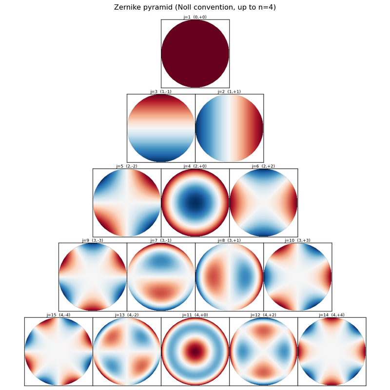
generate_pyramid_image.py renders the canonical Noll pyramid (basis functions themselves, not any wafer data). Independent of the three-stage demo. Run it when you need a fresh reference image for docs or slides.
python generate_pyramid_image.py --with_namesOutputs zernike_pyramid.png in the script’s folder by default. Key CLI options: --n_max (default 4 → 15 terms), --with_names (Piston/Tilt X/… labels), --output_folder, --output_file, --cmap. See -h for the full list.
wlzpoly.reconstruct is the inverse of decompose: it pushes the fitted Zernike coefficients back through the basis matrix to recover the N-point measurement profile (T = A·a). No ground-truth comparison and no R² — intended for production / inference use where the true T is unknown.
python -m wlzpoly.reconstruct `
    --input_folder . `
    --wafer_point_json ./1_samples/points_13.json `
    --decomposed_file ./2_decomposition/decomposed_targets_lsq.csv `
    --output_folder ./4_reconstruction `
    --output_file reconstructed_lsq.csv `
    --n_terms 9 `
    --col_wafer_id id
Output: 4_reconstruction/reconstructed_lsq.csv (id + P1..PN, same wide shape as Stage 1’s target_file.csv). The reconstruct() Python API returns a pd.DataFrame only — the CLI handles CSV writing.
                  ┌────────────────────────┐
                  │  configuration/        │
                  │   config.json          │
                  │   points_13.json       │
                  └────────────┬───────────┘
                               │
                               ▼
                  ┌────────────────────────┐
                  │ generate_samples.py    │  Stage 1
                  └────────────┬───────────┘
                               │
                               ▼
                  ┌────────────────────────┐
                  │  1_samples/            │  target_file.csv +
                  │                        │  ground_truth.csv +
                  │                        │  points_13.json (copy)
                  └─────────┬──────────────┘
                            │  target_file + wafer_points
              ┌─────────────┴──────────────┐
              │                            │
              ▼                            ▼
    ┌──────────────────┐         ┌──────────────────┐
    │ decompose.py     │ Stage 2 │ decompose.py     │ Stage 2
    │  --solver lsq    │         │  --solver ridge  │
    │                  │         │   --auto_lam     │
    └────────┬─────────┘         └────────┬─────────┘
             │                            │
             ▼                            ▼
    ┌─────────────────────────────────────────────┐
    │  2_decomposition/                           │
    │   decomposed_targets_lsq.csv                │
    │   decomposed_targets_ridge.csv              │
    └──────────┬──────────────────────────┬───────┘
               │                          │
               │ + ground_truth.csv       │ + wafer_point_json
               │   (from 1_samples)       │   (basis A)
               ▼                          ▼
       ┌──────────────┐           ┌──────────────────┐
       │  verify.py   │  Stage 3  │ reconstruct.py   │  Stage 4
       │ (no fitting) │           │ (T_recon = A·a)  │
       └──────┬───────┘           └────────┬─────────┘
              │                            │
              ▼                            ▼
      ┌──────────────────┐         ┌──────────────────┐
      │ 3_verification/  │         │ 4_reconstruction/│
      └──────────────────┘         └──────────────────┘
Zernike polynomial library. Follows the Noll convention; the j → (n, m) mapping is computed dynamically by the standard algorithm, so any radial order is supported.
ZernikePolynomials exposes three usage modes:
Operations independent of any specific coefficient set. Call as ZernikePolynomials.method().
| Method | Purpose |
|---|---|
ZernikePolynomials.nm_from_noll(j) |
Noll index j → (n, m) |
ZernikePolynomials.radial(n, m, rho) |
Radial polynomial R_n^m(ρ) |
ZernikePolynomials.basis(j, rho, theta) |
Z_j(ρ, θ) |
ZernikePolynomials.basis_matrix(rho, theta, n_terms=…) |
Design matrix A for fitting |
ZernikePolynomials.to_polar(x=…, y=…) |
Cartesian → polar (r, theta_rad) |
ZernikePolynomials.to_cartesian(r=…, theta=…) |
Polar → Cartesian (x, y) |
ZernikePolynomials.pyramid_image(n_max=…, names=…, return_type='png'|'figure') → Union[bytes, Figure] |
Zernike pyramid image (PNG bytes or Figure) |
An instance carrying a coefficient set — i.e. “this particular wafer/wavefront expressed as a Zernike expansion”.
z = ZernikePolynomials(coeffs={1: 500.0, 4: -12.0, 6: 0.5}, n_terms=9)
# Or
z = ZernikePolynomials(coeffs=[500.0, 0.5, -0.3, -2.0, 0.1, 0.2, 0, 0, 0])  # array OK

# Evaluation
field = z.evaluate(rho=rho, theta=theta)  # ndarray

# Indexing / metadata
z[4]                # -12.0 (a_4)
z[99]               # 0.0 (undefined j returns 0)
len(z)              # 9 (n_terms)
repr(z)             # "ZernikePolynomials(n_terms=9, a1=500.000, dominant=a4=-12.000)"
z.rms()             # sqrt(sum a_j^2), piston excluded by default
z.rms(exclude_piston=False)
For a wafer heatmap (with measurement-point overlay) use WaferLevelZernikePolynomials.draw_field(coeffs=…).
Why split it out: basis() and nm_from_noll() are pure math that doesn’t need a coefficient set, so they live at class level. evaluate() and rms() require a specific coefficient set and are therefore instance methods. Visualization (draw_field) only makes sense once measurement-point coordinates are known, so it lives on WaferLevelZernikePolynomials.
A wafer-aware subclass of ZernikePolynomials. It accepts a measurement-point coordinate frame (coords_df), pre-computes the basis matrix A once, then fits per-wafer coefficients from a measurement DataFrame (df_measured).
from wlzpoly.decompose import load_wafer_coordinates, load_measured_data
from wlzpoly import WaferLevelZernikePolynomials

coords_df = load_wafer_coordinates(
    wafer_points_file="points_13.json", coordinate="cartesian",
)
df_measured = load_measured_data(target_file="1_samples/target_file.csv")

wlz = WaferLevelZernikePolynomials(
    coords_df=coords_df,
    coordinate="cartesian",
    n_terms=9,
)
# wlz.A : np.ndarray (m × n_terms) — pre-computed basis
fit_results = wlz.fit_coefficients(
    mesured_df=df_measured, solver="lsq",
)
# fit_results : list of {"id": <wafer_id>, "coeffs": np.ndarray}

# Render one wafer's fitted wavefront (heatmap + measurement points)
fig = wlz.draw_field(coeffs=fit_results[0]["coeffs"])
fig.savefig("W_01_fit.png", dpi=130, bbox_inches="tight")
Why split it out: the base ZernikePolynomials covers “coefficients are already known” scenarios (sample generation, ground truth), while WaferLevelZernikePolynomials covers the “coordinates + measurements → fitted coefficients” scenario. Two distinct responsibilities.
This module does not read any external files (no config dependency).
Pyramid usage example:
import json
from pathlib import Path
from wlzpoly import ZernikePolynomials

# (n, m) → name mapping is sourced from config.json (optional)
cfg = json.loads(Path("config.json").read_text())
names = {
    tuple(int(x) for x in k.split(",")): v
    for k, v in cfg["zernike_names"].items()
}

# Default return_type='png' → bytes ready to write
png_bytes = ZernikePolynomials.pyramid_image(
    n_max=4,                          # n=0..4 (15 terms total)
    names=names,                      # cell labels (j, n, m only when omitted)
)
Path("zernike_pyramid.png").write_bytes(png_bytes)

# Or get the live Figure for further customization
fig = ZernikePolynomials.pyramid_image(
    n_max=4, names=names, return_type='figure',
)
fig.savefig("zernike_pyramid.png", dpi=130, bbox_inches="tight")
Each cell shows the Noll index j, (n, m), and (when supplied) the optical name. The sign of Z_j(ρ, θ) on the unit disk is rendered with the RdBu_r colormap. return_type selects PNG bytes (for saving / HTML embedding) or a live matplotlib Figure.
General-purpose linear-regression solvers (no Zernike dependency).
Provided functions:
fit_lsq(A, T)— plain least squares: â = (AᵀA)⁻¹ Aᵀ Tfit_ridge(A, T, lam=…)— Ridge: â = (AᵀA + λI)⁻¹ Aᵀ Tloocv_lambda(A, T, lambdas=…)— LOOCV-driven λ selection
wlzpoly.decompose (Stage 2) imports this module.
python generate_samples.py [options]| Option | Default | Description |
|---|---|---|
--noise_sigma, -n |
5.0 | Gaussian noise standard deviation |
--seed, -s |
42 | Random seed |
--n_drift |
30 | Number of wafers in the drift time series |
--working_folder |
Path(__file__).parent |
Base folder for resolving --config_json and --wafer_points |
--config_json |
"config.json" |
Config JSON (resolved under --working_folder if relative) |
--wafer_points |
"wafer_points.json" |
Wafer-points JSON (resolved under --working_folder if relative) |
--output_folder |
Path(__file__).parent / "samples" |
Output folder |
Examples:
python generate_samples.py --noise_sigma 0.4 --seed 100
python generate_samples.py -n 10 --n_drift 50python -m wlzpoly.decompose [options]| Option | Default | Description |
|---|---|---|
--working_folder |
Path.cwd() |
Base folder for resolving --wafer_points |
--wafer_points |
"wafer_points.json" |
Wafer-points JSON (resolved under --working_folder if relative) |
--input_file |
"target_file.csv" |
Measurement CSV (id + P1..PN) |
--n_terms |
9 | Number of Zernike polynomial terms (Noll j=1..n_terms); must be ≤ number of measurement points |
--output_folder |
Path.cwd() / "decomposition" |
Output folder |
--output_file |
"decomposed_targets.csv" |
Filename for the fitted-coefficients CSV (written inside --output_folder) |
--solver |
lsq | lsq or ridge |
--lam |
0.01 | Ridge regularization (used when solver=ridge AND --auto_lam is NOT set) |
--auto_lam |
off | When set with --solver ridge, picks λ via LOOCV (--lam ignored) |
--loocv_lambdas |
[0.0, 0.001, 0.01, 0.1, 1.0, 10.0, 100.0] |
Candidate λ values for LOOCV (when --auto_lam) |
--loocv_ref |
first_wafer |
LOOCV reference T: first_wafer / mean / per_wafer |
--coordinate |
cartesian | cartesian (read x, y) or polar (read r, theta) |
--col_wafer_id |
"wafer_id" |
Name of the wafer-id column in --input_file (also used as id column in output CSV) |
--col_points |
P1 P2 … P13 |
Measurement-point column names in --input_file; must match point ids in --wafer_points |
--coeff_prefix |
"a" |
Prefix for the coefficient columns in the output CSV (<prefix>1..<prefix>n_terms) |
If the columns of --input_file do not match --col_wafer_id / --col_points, or the point ids in the --wafer_points JSON do not match --col_points, parse_args() aborts immediately with parser.error before main runs.
python -m wlzpoly.verify [options]| Option | Default | Description |
|---|---|---|
--decomposed_lsq_file |
"decomposed_targets_lsq.csv" |
LSQ CSV from Stage 2 (id + a1..aN). Skipped if file missing |
--decomposed_ridge_file |
"decomposed_targets_ridge.csv" |
Ridge CSV from Stage 2. Skipped if file missing |
--ground_truth_file |
"ground_truth_file.csv" |
Ground-truth CSV (id, scenario, a1..aN) |
--n_terms |
9 | Number of Zernike polynomial terms (must match Stage 2 run) |
--scenarios_to_show |
auto (all non-drift scenarios) |
Scenario labels to include in per-scenario tables/charts |
--output_folder |
Path.cwd() / "verification" |
Output folder |
python -m wlzpoly.reconstruct [options]CLI options are split into two argparse groups (Input / Output); -h displays them under those headings.
Input
| Option | Default | Description |
|---|---|---|
--input_folder |
Path.cwd() |
Base folder for resolving --wafer_point_json |
--wafer_point_json |
"wafer_points.json" |
Wafer-points JSON (must have .json extension; resolved under --input_folder if relative) |
--decomposed_file |
"decomposed_targets.csv" |
Decomposed-coefficients CSV (id + <prefix>1..<prefix>N) |
--n_terms |
9 | Number of Zernike terms to read from --decomposed_file. Must equal the count of <prefix>\d+ columns in the CSV |
--coordinate |
cartesian | cartesian (read x, y) or polar (read r, theta) |
--col_wafer_id |
"wafer_id" |
Name of the wafer-id column in --decomposed_file (also used as id column in output CSV) |
--col_points |
P1 P2 … P13 |
Output measurement-point column names; subset/permutation of --wafer_point_json point ids |
--coeff_prefix |
"a" |
Prefix for the coefficient columns in --decomposed_file |
--coeff_suffix |
"" |
Optional trailing tag on the coefficient columns (e.g. _pred / _true produced by ML-pipeline train_output / test_output CSVs). Columns are read as <prefix><j><suffix> and stripped to bare <prefix><j> internally. Empty by default (matches wlzpoly.decompose output) |
Output
| Option | Default | Description |
|---|---|---|
--output_folder |
Path.cwd() / "reconstruction" |
Output folder (CSV is written by the CLI; reconstruct() API only returns the DataFrame) |
--output_file |
"reconstructed_targets.csv" |
Filename for the reconstructed-measurements CSV |
parse_args() aborts with parser.error if any of the following are violated: --wafer_point_json does not end in .json; --decomposed_file or --wafer_point_json does not exist; --decomposed_file is missing the required --col_wafer_id / <coeff_prefix>1<coeff_suffix>..<coeff_prefix>N<coeff_suffix> columns; the number of <coeff_prefix>\d+<coeff_suffix> columns in --decomposed_file does not equal --n_terms; any of --col_points is not present in the --wafer_point_json point ids.
points_13.json stores both (x, y) and (r, theta) for the same 13 points. On a few diagonal edge points the stored r=145 is rounded (the exact value is √(102.5² + 102.5²) = 144.957).
--coordinate cartesian(default): read only (x, y) from JSON; convert to polar via theZernikePolynomials.to_polar(x=…, y=…)classmethod, which usesarctan2and is numerically exact.--coordinate polar: read only (r, theta) from JSON. Theta is stored in degrees and converted withnp.deg2rad.
The RMSE difference between the two modes is at the 4th-decimal level (e.g. a1 LSQ: cartesian 1.5461 vs polar 1.5465). The flag exists so the consumer chooses which JSON field to trust explicitly. decompose.py‘s load_wafer_coordinates() / load_measured_data() and the WaferLevelZernikePolynomials class are reused by verify.py.
Used only by generate_samples.py (Stage 1) for synthetic-data generation. wlzpoly.decompose and wlzpoly.verify do not read it — their per-run knobs (n_terms, loocv_lambdas, scenarios_to_show) are CLI flags instead.
{
  "wafer": {
    "size_mm": 300,
    "edge_exclusion_mm": 5,
    "fit_radius_mm": 145
  },

  "scenarios": {
    "normal":     {"1": 500.0, "2": 0.5, ..., "9": 0.0},
    "tilted":     {"1": 498.0, "2": 8.0, ...},
    "bowl":       {...},
    "astigmatic": {...},
    "trefoil":    {...},
    "comatic":    {...}
  },

  "drift_series": {
    "piston_decay_per_step": -0.15,
    "bowl_deepen_per_step":  -0.10,
    "piston_random_sigma":    0.4,
    "bowl_random_sigma":      0.3,
    "shape_random_sigma":     0.2
  },

  "decomposition": {
    "n_terms": 9,
    "loocv_lambdas": [0.0, 0.001, 0.01, 0.1, 1.0, 10.0, 100.0],
    "scenarios_to_show": [
      "normal", "tilted", "bowl",
      "astigmatic", "trefoil", "comatic"
    ]
  },

  "zernike_names": {
    "0,0":  "Piston",
    "1,1":  "Tilt X",
    "1,-1": "Tilt Y",
    ...
  }
}| Section | Used by | Meaning |
|---|---|---|
wafer |
(informational) | Wafer size + edge exclusion + fitting radius |
scenarios |
Stage 1 | Six ground-truth scenarios (a₁..a₉ coefficients) |
drift_series |
Stage 1 | Time-series drift parameters (decay + random walk σ) |
decomposition.n_terms |
Stage 1 | Zernike order for ground-truth generation. Stage 2/3 use --n_terms CLI instead |
decomposition.loocv_lambdas, scenarios_to_show |
(legacy) | No longer read by Stage 2/3 — use --loocv_lambdas / --scenarios_to_show CLI flags |
zernike_names |
(legacy) | No longer read by Stage 2/3 — the standard (n, m) → name map is hardcoded in wlzpoly.verify |
13-point measurement coordinate definition (cardinal-aligned pattern).
{
  "wafer_size_mm": 300,
  "edge_exclusion_mm": 5,
  "wafer_radius_mm": 145,
  "pattern": "13-point cardinal-aligned",
  "points": [
    {"id": "P1",  "x": 0,    "y": 0,    "r": 0,   "theta": 0,   "zone": "Center"},
    {"id": "P2",  "x": 75,   "y": 0,    "r": 75,  "theta": 0,   "zone": "Mid_E"},
    ...
    {"id": "P13", "x": 102.5, "y": -102.5, "r": 145, "theta": 315, "zone": "Edge_SE"}
  ]
}
The 13-point layout:
- P1: Center (1)
- P2..P5: Middle ring r=75mm at 0°/90°/180°/270° (4)
- P6..P13: Edge ring r=145mm at 0°/45°/…/315° (8)
id,P1,P2,P3,...,P13
W_01,504.99,497.06,504.92,...,502.55
W_02,507.97,510.82,493.97,...,506.47
...
13-point thickness measurements — same shape as a real metrology export.
id,scenario,a1,a2,a3,...,a9
W_01,normal,500.0,0.5,-0.3,...,0.0
W_02,tilted,498.0,8.0,-1.5,...,0.0
Per-wafer ground-truth Zernike coefficients (used only for verification).
id,a1,a2,a3,...,a9
W_01,499.27,-1.99,2.16,...,0.21
W_02,498.50,8.05,-1.61,...,-0.05
LSQ-recovered coefficients — the 13 → 9 compression result (production output).
id,scenario,a1_true,a1_lsq,a1_ridge,a2_true,a2_lsq,a2_ridge,...
W_01,normal,500.0,499.27,499.20,0.5,-1.99,-1.95,...
For every coefficient, three columns: truth / LSQ / Ridge → 27 columns + 2 metadata.
Six scenario wafers, one row each. Every row has three panels:
┌──────────────┬───────────────┬─────────────────────────────────┐
│  W_01        │   mean (a1)   │   shape components (a2..a9)    │
│  normal      │   [narrow bar]│   [eight wide bars]             │
└──────────────┴───────────────┴─────────────────────────────────┘
- Left: id + scenario label
- Middle: a₁ (Piston, mean thickness) — y-axis zoomed to ±5
- Right: a₂..a₉ (shape components)
Every bar panel pairs navy (truth) with orange (fitted). The closer the bars overlap, the more accurate the fit.
Per-coefficient RMSE across 36 samples:
coef          RMSE (LSQ)    RMSE (Ridge)
----------------------------------------
a1 (Piston  )    1.5464        1.6408
a2 (Tilt X  )    1.6980        1.6955
...
a9 (Trefoil Y)   0.8764        0.8762

λ used for Ridge: 0.01
id,P1,P2,P3,...,P13
W_01,502.56,495.79,507.85,...,495.94
W_02,503.00,510.27,497.91,...,505.76
...
Same wide shape as target_file.csv from Stage 1 (id + P1..PN). Produced by wlzpoly.reconstruct from a Stage 2 decomposed-coefficients CSV via T_recon = A · a, with no noise added back. The per-point residual target_file − reconstructed_targets is the part that the first N Zernike basis functions could not absorb (noise + truncation error). run_demo.ps1 writes two files — reconstructed_lsq.csv and reconstructed_ridge.csv — mirroring the Stage 2 fits.
Six ground-truth scenarios defined in config.json:
| Scenario | Dominant coefficient | Meaning |
|---|---|---|
| normal | a₄ = -2 | Nominal (mild bowl) |
| tilted | a₂ = +8 | Chuck level error (Tilt X) |
| bowl | a₄ = -12 | Center-to-edge imbalance (deep Defocus) |
| astigmatic | a₆ = +6.5 | Showerhead 0/90 asymmetry |
| trefoil | a₉ = +4.5 | 3-zone heater issue |
| comatic | a₈ = +3.8 | X-direction asymmetric flow |
Total: 36 wafers = 6 scenarios + 30 drift samples (drift = a₁ decay + a₄ deepening + random walk on the others).
Edit run_demo.ps1 Stage 1 line — change --noise_sigma 5.0 to the desired value — then .\run_demo.ps1. Or call manually (run from examples/):
# Low noise (LSQ recovers near-perfectly)
python generate_samples.py --working_folder . \
    --config_json ./configuration/config.json \
    --wafer_points ./configuration/points_13.json \
    --output_folder ./1_samples --noise_sigma 0.4

# Stage 2a: LSQ
python -m wlzpoly.decompose --working_folder . \
    --wafer_points ./1_samples/points_13.json \
    --input_file ./1_samples/target_file.csv \
    --output_folder ./2_decomposition \
    --output_file decomposed_targets_lsq.csv \
    --n_terms 9 --solver lsq

# Stage 2b: Ridge with LOOCV
python -m wlzpoly.decompose --working_folder . \
    --wafer_points ./1_samples/points_13.json \
    --input_file ./1_samples/target_file.csv \
    --output_folder ./2_decomposition \
    --output_file decomposed_targets_ridge.csv \
    --n_terms 9 --solver ridge --auto_lam --loocv_ref first_wafer

# Stage 3
python -m wlzpoly.verify \
    --decomposed_lsq_file ./2_decomposition/decomposed_targets_lsq.csv \
    --decomposed_ridge_file ./2_decomposition/decomposed_targets_ridge.csv \
    --ground_truth_file ./1_samples/ground_truth.csv \
    --n_terms 9 --output_folder ./3_verification

# Stage 4a: LSQ reconstruction
python -m wlzpoly.reconstruct --input_folder . \
    --wafer_point_json ./1_samples/points_13.json \
    --decomposed_file ./2_decomposition/decomposed_targets_lsq.csv \
    --output_folder ./4_reconstruction \
    --output_file reconstructed_lsq.csv \
    --n_terms 9 --col_wafer_id id

# Stage 4b: Ridge reconstruction
python -m wlzpoly.reconstruct --input_folder . \
    --wafer_point_json ./1_samples/points_13.json \
    --decomposed_file ./2_decomposition/decomposed_targets_ridge.csv \
    --output_folder ./4_reconstruction \
    --output_file reconstructed_ridge.csv \
--n_terms 9 --col_wafer_id idAppend to config.json:
"scenarios": {
  ...
  "spherical_issue": {
    "1": 500.0, "2": 0.0, "3": 0.0, "4": -1.0,
    "5": 0.0, "6": 0.0, "7": 0.0, "8": 0.0, "9": 0.0
  }
}
No code change required.
Three places matter:
-
Stage 1 (ground-truth generation): bump
cfg["decomposition"]["n_terms"]inconfig.jsonsoground_truth.csvcarriesa1..a11instead ofa1..a9. -
Stage 2 / 3 (fitting + verification): pass
--n_terms 11on the CLI. The flag is the only authority for the fitter — neither module readsconfig.json. -
Stage 4 (reconstruction): pass the same
--n_terms 11towlzpoly.reconstruct. The CLI rejects any mismatch between--n_termsand the<coeff_prefix>\d+column count in--decomposed_file, so Stages 2 and 4 must agree.
python -m wlzpoly.decompose    ... --n_terms 11
python -m wlzpoly.verify       ... --n_terms 11
python -m wlzpoly.reconstruct  ... --n_terms 11
Maximum n_terms is the number of measurement points (13 here). Exceeding it makes AᵀA singular and the coefficients diverge — leave at least 4 residual DOF for stable fits.
Edit points_13.json directly (coordinates and zones are user-editable). No code change required.
python -m wlzpoly.verify --output_folder my_resultsWafer thickness is modeled as a sum of Zernike polynomials on the unit disk:
T(ρ, θ) = Σ_{k=1..N} a_k · Z_k(ρ, θ) + ε
where:
| Symbol | Meaning |
|---|---|
T(ρ, θ) |
wafer thickness at a point on the unit disk (the quantity being decomposed) |
ρ |
normalized radial coordinate; ρ = 0 at the wafer center, ρ = 1 at the fitting-radius edge |
θ |
azimuthal angle, in radians, measured CCW from the +x axis |
N |
number of Zernike terms retained in the expansion (= the --n_terms CLI flag) |
k |
Noll index, k = 1 .. N |
a_k |
k-th Zernike coefficient (Noll index k), recovered by the fitter |
Z_k(ρ, θ) |
k-th Zernike polynomial in the Noll convention |
ε |
measurement noise (per-point residual not captured by the first N basis functions) |
Sampled at the 13 measurement points, this becomes a linear system:
T = A · a + ε (T: 13×1, A: 13×9, a: 9×1)
where:
| Symbol | Shape | Meaning |
|---|---|---|
T |
13×1 | measured thickness vector; T[i] = thickness at measurement point i |
A |
13×9 | basis matrix; A[i, k] = Z_k(ρ_i, θ_i) — k-th Zernike polynomial evaluated at the i-th measurement point |
a |
9×1 | Zernike coefficient vector; a[k] = a_k, the unknown to be recovered by the fitter |
ε |
13×1 | per-point measurement noise (residual not captured by the first 9 basis functions) |
13 |
— | number of measurement points (= rows of A and T); set by --wafer_points JSON |
9 |
— | number of Zernike terms (= columns of A = rows of a); set by --n_terms (default 9) |
Reconstruction is the inverse of decomposition: given an already-known Zernike coefficient vector a, regenerate the N-point measurement profile it describes. This is what wlzpoly.reconstruct (Stage 4, optional) does.
T_recon = A · a (no ε; reconstructed signal is noise-free by construction)
where:
| Symbol | Shape | Meaning |
|---|---|---|
T_recon |
13×1 | reconstructed thickness vector at the same N measurement points |
A |
13×9 | same basis matrix as in decomposition (A[i, k] = Z_k(ρ_i, θ_i)) |
a |
9×1 | fitted (or otherwise known) Zernike coefficient vector |
Per measurement point i, the reconstructed thickness is the inner product of basis row i with the coefficient vector:
T_recon[i] = a_1 · Z_1(ρ_i, θ_i)
           + a_2 · Z_2(ρ_i, θ_i)
           + ...
           + a_N · Z_N(ρ_i, θ_i)
           = Σ_k  A[i, k] · a_k
Stacking all 13 rows gives T_recon = A · a. For many wafers at once, the implementation runs one matrix multiply T_matrix = a_matrix @ A.T so the output shape is (n_wafers, n_points).
Tiny worked example (illustrative A values, not the real Zernike values; n_terms=3, n_points=4):
a = [500.0, 2.0, 0.5]       # piston, tilt-x, defocus
A = [[1.0,  0.0, -1.0],     # row per measurement point
     [1.0,  1.0,  0.0],
     [1.0,  0.0,  1.0],
     [1.0, -1.0,  0.0]]
T_recon = A · a
        = [1.0·500 + 0.0·2 + (-1.0)·0.5,    # = 499.5
           1.0·500 + 1.0·2 +  0.0·0.5,      # = 502.0
           1.0·500 + 0.0·2 +  1.0·0.5,      # = 500.5
           1.0·500 + (-1.0)·2 + 0.0·0.5]    # = 498.0
Comparison with decomposition:
| Direction | Knowns | Unknown | Cost |
|---|---|---|---|
| Decompose (Stage 2) | T (measured) + A (geometry) | a — recover via LSQ / Ridge | inversion / regularization per wafer |
Reconstruct (wlzpoly.reconstruct) |
a (fitted) + A (geometry) | T_recon — compute directly | one matrix multiply (no fitting) |
Reconstruction never recovers the original noise ε; the residual T − T_recon is the part the first N Zernike terms could not absorb.
| Solver | Formula | Properties |
|---|---|---|
| LSQ | â = (AᵀA)⁻¹ Aᵀ T | Unbiased, higher variance |
| Ridge | â = (AᵀA + λI)⁻¹ Aᵀ T | Biased toward zero, lower variance |
The hat on â is the standard statistics convention for estimate of the unknown true value — here, the estimate of the true coefficient vector a recovered from the measurements.
The CLI flag --lam directly supplies λ in the Ridge formula (i.e. --lam = λ). For Ridge, λ can be fixed via --lam or chosen automatically with --auto_lam (see next section).
LSQ derivation — minimize the residual sum of squares:
J(a) = ‖T − A·a‖²  =  (T − A·a)ᵀ (T − A·a)

∂J/∂a = −2 Aᵀ (T − A·a) = 0
      ⇒  Aᵀ A · a = Aᵀ T
      ⇒  â = (Aᵀ A)⁻¹ Aᵀ T
Ridge derivation — same loss as LSQ plus a coefficient-size penalty:
J(a) = ‖T − A·a‖² + λ ‖a‖²

∂J/∂a = −2 Aᵀ (T − A·a) + 2 λ a = 0
      ⇒  (Aᵀ A + λI) · a = Aᵀ T
      ⇒  â = (Aᵀ A + λI)⁻¹ Aᵀ T
The only structural difference is the λI added on the diagonal of AᵀA, which (a) makes the matrix invertible even when AᵀA is rank-deficient, and (b) shrinks the coefficients toward zero (bias) in exchange for lower variance.
When wlzpoly.decompose --solver ridge --auto_lam is set, λ is picked by Leave-One-Out Cross-Validation instead of being supplied as a fixed --lam.
Inputs:
A— basis matrix (N measurement points × n_terms columns)T— a measurement vector for one wafer (length N)λcandidates —--loocv_lambdas(default[0.0, 0.001, 0.01, 0.1, 1.0, 10.0, 100.0])
Algorithm (for each candidate λ):
for i in 0..N-1:                              # N folds
    A_train = A with row i removed            # (N-1) × n_terms
    T_train = T with element i removed        # (N-1)
    â = (A_trainᵀ A_train + λI)⁻¹ A_trainᵀ T_train
    pred_i  = A[i, :] @ â                     # predict the held-out point
    err_i   = T[i] - pred_i

mean_err²(λ) = mean( err_i² for i in 0..N-1 )

best_λ = argmin_λ  mean_err²(λ)
Each λ candidate is scored by how well an N-1 fit predicts the left-out point, averaged over all N folds. Small λ → overfits noise, leave-out predictions bad. Large λ → kills signal, leave-out predictions bad. The minimum-error λ is the sweet spot.
Which T to scan over — --loocv_ref (decompose-only):
| Mode | Behavior | When useful |
|---|---|---|
first_wafer (default) |
LOOCV on the first wafer’s T; that single λ is reused for all wafers | Fast; first wafer is representative of the batch |
mean |
Per-point mean across all wafers; single λ for all | Single outlier wafer shouldn’t dominate λ choice |
per_wafer |
Run LOOCV per wafer; each wafer gets its own λ | Most accurate, N× slower; wafers have very different noise |
Effect on coefficients: in the bundled demo (36 wafers, σ=5.0 noise) LOOCV consistently picks λ = 0.01, which is the same value as the fixed --lam default — so LSQ and Ridge RMSE are within 5%. With higher noise (σ ≥ 10) Ridge with LOOCV-picked λ noticeably outperforms LSQ on edge-of-disk coefficients (a₇..a₉).
| Group | Coefficient(s) | Meaning |
|---|---|---|
| W2W (Wafer-to-Wafer) | a₁ (Piston) | Mean thickness |
| WiW (Within-Wafer) | a₂..a₉ | Spatial pattern (8 modes) |
Sanity check: 13 measurements → 9 coefficients → 4 residual DOF (used for residual monitoring).
Python 3.9+
numpy >= 1.22
pandas >= 1.5
matplotlib >= 3.5
tqdm >= 4.60
Standard-library only beyond those: argparse, csv, json, math, pathlib, typing.