
@wolf
Forum Replies Created
-
AuthorPosts
-

SHF의 Motto
“Avoir une autre langue, c’est posséder une deuxième âme.”
“다른 언어를 갖는다는 것은 두 번째 영혼을 갖는 것이다.”American Association of Teachers of French
Motto: a guiding principle, a guiding phrase, a core belief expressed in a short phrase, a phrase that expresses the group’s values-
This reply was modified 2 months, 4 weeks ago by Wolf.
-
This reply was modified 2 months, 4 weeks ago by
 yRocket.
-
This reply was modified 2 months, 4 weeks ago by yRocket.
Optimizing the Model: Maximum Likelihood Estimation (MLE)
In Bayesian Optimization, we don’t just “guess” the noise $\sigma_{n}^{2}$ or the kernel lengthscale $l$. We find the values that make our observed data most probable. This process is called tuning the hyperparameters of the Gaussian Process.
1. The Marginal Log-Likelihood (MLL)
To find the best parameters (collectively called $\theta$), we maximize the Marginal Log-Likelihood. This function tells us how well our GP model explains the data we have already collected.
For a set of observations $y$ at points $X$, the Log-Likelihood is defined as:
$$\log p(y|X, \theta) = \underbrace{-\frac{1}{2} y^{T} \tilde{K}^{-1} y}_{\text{Data Fit}} – \underbrace{\frac{1}{2} \log |\tilde{K}|}_{\text{Complexity Penalty}} – \underbrace{\frac{n}{2} \log 2\pi}_{\text{Constant}}$$
Where $\tilde{K} = K_{\theta} + \sigma_{n}^{2}I$.
2. The Tug-of-War: Fit vs. Complexity
The MLE formula is a beautiful balancing act between two competing forces:
A. The Data Fit Term ($-\frac{1}{2} y^{T} \tilde{K}^{-1} y$)
This term rewards parameters that make the model pass close to the data points.
* If the lengthscale $l$ is very short, the model can “wiggle” to hit every point perfectly, making this term very high.B. The Complexity Penalty ($-\frac{1}{2} \log |\tilde{K}|$)
This term (the determinant of the covariance matrix) penalizes models that are too complex or “wiggly.”
* It prefers a simple, smooth line over a jagged one.
* As $l$ gets smaller (more complex), this penalty grows.
3. How the Optimizer Finds $\sigma_{n}^{2}$ and $l$
The AI learner should visualize the MLE process as a separate “mini-optimization” inside the BO loop:
- Start: Pick initial values for $l$ and $\sigma_{n}^{2}$.
- Calculate: Compute the Log-Likelihood using the formula above.
- Gradient Ascent: Calculate the derivative of the Likelihood with respect to the parameters and “climb” the hill to find the peak.
- Update: Set the GP to use these optimized parameters for the next prediction.
4. Why MLE makes BO Robust
By using MLE, the Bayesian Optimizer self-corrects:
* If the data is noisy: The MLE will naturally increase $\sigma_{n}^{2}$ to avoid the “Complexity Penalty” of trying to fit every noise spike.
* If the function is simple: The MLE will increase the lengthscale $l$, allowing the model to share information across much larger distances.Summary for the Learner
Parameter If too small… If too large… Lengthscale ($l$) Overfits (too wiggly) Underfits (too flat) Noise ($\sigma_{n}^{2}$) Mistrusts the trend (sees noise as signal) Ignores the data (sees signal as noise)
Incorporating Noise ($\epsilon$) into the Matrix Calculation
In real-world applications (like lab experiments or noisy sensor data), we rarely get the “perfect” value. Every time we measure $y$, we are actually seeing the true function value $f(x)$ plus some random noise $\epsilon$.
Mathematically, we model this as:
$$y = f(x) + \epsilon, \quad \epsilon \sim N(0, \sigma_{n}^{2})$$To make Bayesian Optimization robust to this messiness, we must adjust our Covariance Matrix calculation.
1. The Regularized Covariance Matrix
When data is noisy, we no longer want the Surrogate Model to pass exactly through every data point (which would be overfitting the noise). Instead, we add a “noise term” to the diagonal of our training covariance matrix $K$.
The noisy covariance matrix $\tilde{K}$ is defined as:
$$\tilde{K} = K + \sigma_{n}^{2} I$$Where:
* $K$: The original kernel covariance matrix.
* $\sigma_{n}^{2}$: The variance of the noise (how “messy” the data is).
* $I$: The Identity Matrix (a matrix with 1s on the diagonal and 0s elsewhere).$$ \tilde{K} = \begin{pmatrix}
k(x_{1}, x_{1}) + \sigma_{n}^{2} & k(x_{1}, x_{2}) & \cdots \cr
k(x_{2}, x_{1}) & k(x_{2}, x_{2}) + \sigma_{n}^{2} & \cdots \cr
\vdots & \vdots & \ddots
\end{pmatrix} $$
2. Updated Uncertainty with Noise
When we predict the uncertainty $\sigma^{2}(x_{\ast})$ at a new point using this noisy matrix, the formula becomes:
$$\sigma^{2}(x_{\ast}) = K_{\ast\ast} – K_{\ast}^{T} (K + \sigma_{n}^{2}I)^{-1} K_{\ast}$$
What changes for the AI learner?
1. Non-Zero Uncertainty at Observed Points: In a noiseless GP, $\sigma$ drops to exactly 0 at a tested point. With noise, the uncertainty at a tested point stays slightly above zero because the model knows the measurement itself might be slightly off.
2. Smoothing Effect: The mean prediction $\mu(x_{\ast})$ no longer has to “touch” every blue dot. It creates a smooth path that averages the noise, leading to more stable optimization.
3. Impact on the Acquisition Function
In noisy environments, the Acquisition Function becomes more “cautious.”
* Without noise, BO might find a huge “spike” in the data and assume it found the global maximum.
* With noise modeling, BO realizes that a single high point might just be a “lucky” noise artifact. It will often require multiple samples in a promising area to “confirm” that the peak is real.
4. Summary of the “Identity Matrix” Trick
By adding $\sigma_{n}^{2}$ to the diagonal (often called Tikhonov regularization or a Nugget term):
* We prevent numerical instability (it makes the matrix easier to invert).
* We tell the AI: “Trust the general trend, not the individual points.”
* We ensure the global minimum search isn’t distracted by outliers.
Calculating Uncertainty ($\sigma$) in Gaussian Processes
The “Uncertainty” in Bayesian Optimization comes from the Conditional Variance of the Gaussian Process. When we observe data, the GP uses the Kernel’s covariance matrix to “pinch” the uncertainty at those points, while letting it grow in unobserved regions.
1. Defining the Components
Assume we have already tested $n$ points, which we call our training set $X$. We now want to predict the value and uncertainty at a new, untested point $x_{\ast}$.
We use three components derived from our Kernel function $k(x, x’)$:
* $K$: The $n \times n$ covariance matrix of the training points $X$.
* $K_{\ast}$: An $n \times 1$ vector of covariances between the training points $X$ and the new point $x_{\ast}$.
* $K_{\ast\ast}$: The scalar covariance of the new point $x_{\ast}$ with itself (the “prior” variance).
2. The Uncertainty Formula
The uncertainty (variance) at the new point, denoted as $\sigma^{2}(x_{\ast})$, is calculated by subtracting the “information we gained” from the “initial uncertainty.”
$$\sigma^{2}(x_{\ast}) = K_{\ast\ast} – K_{\ast}^{T} K^{-1} K_{\ast}$$
Breaking down the math:
- $K_{\ast\ast}$ (Prior Uncertainty): This is the maximum uncertainty we have about any point before seeing data. For an RBF kernel, this is usually $\sigma_{f}^{2}$.
- $K_{\ast}^{T} K^{-1} K_{\ast}$ (Information Gain): This term represents how much the points we’ve already seen ($X$) tell us about the new point ($x_{\ast}$).
- If $x_{\ast}$ is very close to a training point, $K_{\ast}$ will have high values.
- The subtraction will be large, making the resulting $\sigma^{2}(x_{\ast})$ very small (near zero).
- If $x_{\ast}$ is very far from all training points, $K_{\ast}$ will be near zero, and the uncertainty will remain high (near $K_{\ast\ast}$).
3. Visualizing the “Pinch”
When we calculate this for every possible $x_{\ast}$ across the search space, we get the famous “confidence envelope” seen in GP plots.
- At Training Points: $\sigma(x)$ drops to 0 (or the level of noise $\sigma_{n}^{2}$ if specified).
- Between Points: $\sigma(x)$ arches upward like a bridge, representing the growing uncertainty as we move away from known data.
4. Why this matters for BO
The Acquisition Function uses this specific $\sigma(x_{\ast})$ to decide where to go next. For example, in Upper Confidence Bound (UCB), the score is:
$$UCB(x) = \mu(x) + \kappa \sigma(x)$$- If $\sigma(x)$ is high, the score increases, forcing the “AI” to go and explore that area to reduce its ignorance.
- This calculation is the exact reason why BO is robust to a lack of data; it knows exactly how much it doesn’t know.
Is Bayesian Optimization (BO) Robust to a Lack of Data?
The short answer is yes. In fact, robustness to small datasets is the primary reason researchers choose Bayesian Optimization over other methods. While Deep Learning requires thousands of data points, BO is specifically designed to perform well with as few as 10 to 50 samples.
1. Why BO Excels with Sparse Data
BO handles “data poverty” through three specific mathematical mechanisms:
A. The Power of the Prior
In traditional statistics, if you have no data, you know nothing. In BO, you start with a Prior (usually a Gaussian Process).
* The Prior defines your assumptions about the function’s “smoothness” and “variance” before any testing begins.
* Even with zero data points, the GP provides a baseline expectation across the entire search space.B. Quantifying “What We Don’t Know”
Most models (like Linear Regression or Neural Networks) provide a single point prediction. If data is sparse, these models often “overfit” or give wildly confident but wrong answers.
BO provides a Mean ($\mu$) and Uncertainty ($\sigma$). When data is missing in a specific region, the uncertainty $\sigma$ naturally increases.C. Informed Exploration
Because BO knows where its data is “thin,” the Acquisition Function can purposefully target those empty regions. It doesn’t guess randomly; it mathematically identifies the point that will provide the most information gain.
2. The Limits of Robustness
While BO is robust, “lack of data” can still cause issues if the search space is too large. This is known as the Curse of Dimensionality.
Scenario Robustness Level Why? Low Dim (1-5 variables) | Low Data Very High GP can easily map the correlations and find the peak. High Dim (20+ variables) | Low Data Low The volume of the search space grows exponentially; 10 points in a 20D space is like 10 drops of water in an ocean. Noisy Data | Low Data Medium The GP can filter noise, but with very few points, it may struggle to distinguish noise from the true signal.
3. How to Improve Robustness with Tiny Datasets
If you are forced to work with extremely limited data (e.g., only 5-10 trials), you can “help” the BO algorithm by:
- Choosing a Strong Kernel: Using a Matérn Kernel instead of RBF can be more robust if you expect the function to have sudden changes rather than perfect smoothness.
- Narrowing Bounds: Don’t search from 0 to 1,000 if you know the answer is likely between 10 and 20.
- Hyperparameter Priors: Instead of letting the GP “learn” the lengthscale $l$ from scratch, you can provide a “Prior” for the lengthscale based on domain knowledge.
4. Summary for the Learner
Bayesian Optimization is the gold standard for small-data optimization. It doesn’t just “survive” a lack of data; it uses the lack of data (uncertainty) as a compass to find the global minimum more efficiently than any other method.
The Role of the Kernel in Bayesian Optimization
In Bayesian Optimization, we don’t just treat points as isolated data. We assume the function is “smooth.” The Kernel function (or Covariance function) $k(x, x’)$ is the mathematical engine that defines this smoothness, allowing the model to “share” information from a tested point to its neighbors.
1. The RBF (Radial Basis Function) Kernel
The RBF kernel (also known as the Squared Exponential kernel) is the most popular choice. It assumes that if two points $x$ and $x’$ are close in the input space, their function values $f(x)$ and $f(x’)$ are highly correlated.
The formula is defined as:
$$k(x, x’) = \sigma_{f}^{2} \exp\left( -\frac{|x – x’|^{2}}{2l^{2}} \right)$$Where:
* $\sigma_{f}^{2}$ (Signal Variance): Controls the vertical scale (how much the function fluctuates).
* $l$ (Lengthscale): Controls the horizontal scale (how far the influence of a point reaches).
2. How Information is Shared
When we use a Gaussian Process (GP) as our surrogate model, we define a Covariance Matrix $K$ for a set of points ${x_{1}, …, x_{n}}$:
$$K = \begin{pmatrix}
k(x_{1}, x_{1}) & k(x_{1}, x_{2}) & \cdots & k(x_{1}, x_{n}) \cr
k(x_{2}, x_{1}) & k(x_{2}, x_{2}) & \cdots & k(x_{2}, x_{n}) \cr
\vdots & \vdots & \ddots & \vdots \cr
k(x_{n}, x_{1}) & k(x_{n}, x_{2}) & \cdots & k(x_{n}, x_{n})
\end{pmatrix}$$The Mechanism:
1. If you evaluate the function at $x_{1}$ and find a high value, the Kernel tells the model: “Because $x_{2}$ is near $x_{1}$, its value is likely high too.”
2. The correlation decreases exponentially as the distance $|x – x’|$ increases.
3. This creates the “smooth” hills and valleys in the surrogate model, allowing BO to predict values in unexplored regions.
3. Comparing Kernels
Different kernels allow BO to share information in different ways:
Kernel Name Formula Concept Behavior RBF Exponential of squared distance Very smooth, infinitely differentiable. Matérn Incorporates Bessel functions Less smooth; better for modeling physical processes with “rougher” changes. Periodic $k(x, x’) = \exp(-\frac{2\sin^{2}(\pi|x-x’|/p)}{l^{2}})$ Shares info across repeating patterns (e.g., seasonal sales).
4. Summary for the Learner
The Kernel is the Prior Knowledge you give to the AI.
* A short lengthscale ($l$) means “only trust data points that are very close.”
* A long lengthscale ($l$) means “one data point tells me a lot about a wide area of the map.”By tuning these kernel parameters (often via Maximum Likelihood Estimation), the Bayesian Optimizer learns exactly how much it can generalize from each expensive test run.
Global Minimum Search: Bayesian Optimization (BO) vs. Gradient Descent (GD)
For an AI learner, understanding the difference between these two is about understanding information. GD uses local “slope” information, while BO uses global “uncertainty” information.
1. Conceptual Framework
Gradient Descent (GD) is a local search algorithm. It calculates the derivative of the loss function $f$ at the current point $x_{n}$ and moves in the direction of the steepest descent.
$$x_{n+1} = x_{n} – \eta \nabla f(x_{n})$$
If the landscape has multiple valleys, GD will simply fall into the closest one.Bayesian Optimization (BO) is a global search strategy. It treats the objective function as a random variable and maintains a posterior distribution over possible functions. It doesn’t just ask “where is the slope pointing?” but “where is the best point likely to be, given everything I’ve seen so far?”
2. Comparison Table
Feature Gradient Descent (GD) Bayesian Optimization (BO) Search Scope Local (Point-to-point) Global (Area-to-area) Information Used Gradient (First-order derivative) Surrogate Model & Acquisition Function Global Minima Capability High risk of trapping in Local Minima High capability via Exploration Function Type Must be differentiable ($f \in C^{1}$) Black-box (No derivative needed) Computational Cost Low per iteration | High total (many steps) High per iteration | Low total (few steps)
3. The Mathematics of Global Search
Gradient Descent and Local Minima
GD relies on the local Taylor expansion. Because it only sees the immediate neighborhood, it converges to a point $x_{\ast}$ where $\nabla f(x_{\ast}) = 0$. In non-convex optimization, there is no guarantee that $f(x_{\ast})$ is the global minimum.
Bayesian Optimization and the Surrogate
BO uses a Gaussian Process (GP) to model the function. For any input $x$, the GP provides a mean $\mu(x)$ and a variance $\sigma^{2}(x)$.
The search for the global minimum is guided by an Acquisition Function, such as Expected Improvement (EI):
$$EI(x) = E[max(f(x_{best}) – f(x), 0)]$$
By evaluating points where the variance $\sigma(x)$ is high, BO explicitly forces the search to leave local valleys and explore unknown territory, effectively “jumping” out of local minima.
4. When to Use Which?
- Use Gradient Descent when you have millions of parameters (like a Neural Network) and the function is “cheap” to evaluate or you have an analytical gradient.
- Use Bayesian Optimization when the function is a “Black Box,” evaluation is extremely “expensive” (e.g., training a model for 10 hours), and you need to find the global best hyperparameters $x_{\ast}$ within a few dozen trials.
The Python Implementation
Each time the code runs an iteration, it updates the Surrogate Model (the Gaussian Process). You can visualize the model getting smarter with every point sampled.
Python
from bayes_opt import BayesianOptimization
import numpy as np

# 1. Define the "Black Box" function we want to maximize
# In reality, this could be a machine learning model training loop
def black_box_function(x, y):
    # This is just a mathematical hill with a peak at (x=2, y=3)
    return -1 * (x - 2)**2 - (y - 3)**2 + 10

# 2. Define the search space (the range for our variables)
pbounds = {'x': (0, 4), 'y': (0, 5)}

# 3. Initialize the Optimizer
# We use a Gaussian Process as the surrogate model by default
optimizer = BayesianOptimization(
    f=black_box_function,
    pbounds=pbounds,
    verbose=2, # 2 prints the steps, 1 only prints the best, 0 is silent
    random_state=1,
)

# 4. Run the Optimization
# init_points: How many random steps to take first (Exploration)
# n_iter: How many Bayesian steps to take (Exploitation)
optimizer.maximize(
    init_points=2,
    n_iter=10,
)

# 5. Get the best result
print("--- Result ---")
print(f"Best parameters: {optimizer.max['params']}")
print(f"Best value found: {optimizer.max['target']}")
Stdout
| iter | target | x | y |
————————————————-
| 1 | 9.528 | 1.668 | 3.602 |
| 2 | 3.787 | 0.0004575 | 1.512 |
| 3 | 6.216 | 0.4351 | 1.844 |
| 4 | 9.613 | 1.415 | 3.213 |
| 5 | 9.288 | 2.649 | 2.461 |
| 6 | 5.842 | 3.724 | 4.09 |
| 7 | 5.908 | 0.459 | 4.31 |
| 8 | 9.307 | 1.753 | 2.205 |
| 9 | 4.449 | 3.095 | 0.9138 |
| 10 | 9.925 | 2.251 | 3.112 |
| 11 | 5.966 | 2.186 | 5.0 |
| 12 | 5.764 | 4.0 | 2.514 |
=================================================
— Result —
Best parameters: {‘x’: 2.250982156847981, ‘y’: 3.111795304557062}
Best value found: 9.92450976682293-
This reply was modified 3 months ago by Wolf.
-
This reply was modified 3 months ago by Wolf.
-
This reply was modified 3 months ago by yRocket.
-
This reply was modified 3 months ago by yRocket.
-
This reply was modified 3 months ago by yRocket.
-
This reply was modified 3 months ago by yRocket.
-
This reply was modified 3 months ago by yRocket.
-
This reply was modified 3 months ago by yRocket.
GP Prior vs. Posterior: The Bayesian View
In Gaussian Processes (GPs), the transition from Prior to Posterior represents the process of “learning” from data. Since a GP is a distribution over functions, this transition describes how our beliefs about which functions are possible change after we observe real data points.
1. The GP Prior (Before seeing data)
The Prior represents our initial assumptions about the function’s behavior (e.g., “it’s smooth,” “it’s periodic,” or “it stays near zero”).
- Definition: We assume the function values $f$ follow a Multivariate Normal Distribution with a mean of zero and a covariance defined by our kernel $K$.
- Visual: If you sample from a GP Prior, you get a “spaghetti” plot of many random, overlapping functions.
- Math: $$f(X) \sim \mathcal{N}(\mathbf{0}, K(X, X))$$
AI Learner Tip: In the Prior, the uncertainty (variance) is the same everywhere. The model has no reason to favor one path over another yet.
2. The GP Posterior (After seeing data)
The Posterior is the updated distribution after we have observed training data $\mathcal{D} = {(x_i, y_i)}$. We “force” the functions to pass through (or near) the observed data points.
- Mechanism: We use Bayes’ Rule:
$$P(f | \text{data}) = \frac{P(\text{data} | f) P(f)}{P(\text{data})}$$ - Result: The “spaghetti” of functions is pruned. Only the functions that are consistent with our observations remain.
- Visual: The functions now “pinch” together at the data points, where uncertainty becomes nearly zero.
3. Key Differences at a Glance
Feature GP Prior GP Posterior Data Involvement None (Assumptions only) Training data incorporated Mean ($\mu$) Usually $\mathbf{0}$ Shifted toward the data points Variance ($\sigma^2$) High and constant ($k(x, x)$) Low near data; High far from data Function Samples Wild and random Constrained to “fit” the observations
4. How the “Learning” Happens
When you move from Prior to Posterior, the GP performs a Joint Distribution calculation. It treats the training points $f$ and the new test point $f_{\ast}$ as part of one big Gaussian vector.
By applying the conditioning rule for Gaussians, the Posterior distribution for a new point $x_{\ast}$ becomes:
$$f_{\ast} | X, f, x_{\ast} \sim \mathcal{N}(\bar{f}_{\ast}, \text{cov}(f_{\ast}))$$
Where the mean $\bar{f}_{\ast}$ is a weighted sum of the training labels $y$, and the variance is reduced because the training data has provided information about the function’s local behavior.
Summary
- Prior: “I think the function is smooth, but I have no idea where it is.”
- Posterior: “I see the data at $x=1$ and $x=2$, so now I’m certain the function passes through those points, though I’m still guessing about $x=10$.”
Calculating $k(x_{\ast}, x_{\ast})$ in Gaussian Processes
To understand how $k(x_{\ast}, x_{\ast})$ is calculated, you have to remember that the Kernel Function (or Covariance Function) is a mathematical rule that defines the relationship between any two points in your input space.
1. The Mathematical Definition
The term $k(x_{\ast}, x_{\ast})$ represents the prior variance at a specific test point $x_{\ast}$. In simpler terms, it answers the question: “Before we see any data, how much do we expect the function value at $x_{\ast}$ to vary?”
If we use the most common kernel, the Squared Exponential (RBF) Kernel, the formula is:
$$k(x, x’) = \sigma_f^2 \exp\left( -\frac{|x – x’|^2}{2\ell^2} \right)$$
When we evaluate this for the same point ($x = x_{\ast}$ and $x’ = x_{\ast}$):
1. The distance $|x_{\ast} – x_{\ast}|^2$ becomes 0.
2. The exponential term $\exp(0)$ becomes 1.
3. Therefore, $k(x_{\ast}, x_{\ast}) = \sigma_f^2$.
2. Physical Interpretation
In a standard GP setup, $k(x_{\ast}, x_{\ast})$ is usually a constant.
Component Interpretation Value It equals the vertical scale variance ($\sigma_f^2$) of your GP. Uncertainty It represents the “Maximum Uncertainty” the model has when it is infinitely far away from any training data. Diagonal Entry In the Joint Covariance Matrix, $k(x_{\ast}, x_{\ast})$ is the diagonal element for the test point.
3. How it fits into the Prediction
Recall the predictive variance formula we discussed earlier:
$$Var(f_{\ast}) = \underbrace{k(x_{\ast}, x_{\ast})}_{\text{Prior Uncertainty}} – \underbrace{K(x_{\ast}, X) K(X, X)^{-1} K(X, x_{\ast})}_{\text{Information Gain from Data}}$$
- Before Data: Your uncertainty is simply $k(x_{\ast}, x_{\ast})$.
- After Data: You subtract a positive value (the second term) based on how much the training data $X$ tells you about $x_{\ast}$.
- At a Training Point: If $x_{\ast}$ is exactly a training point, the second term cancels out the first, and $Var(f_{\ast})$ becomes 0 (assuming no noise).
4. Implementation Example
In Scikit-Learn or GPy, you don’t usually calculate this manually. The library computes the kernel matrix for you:
# Python # Assuming 'gp' is your trained model and 'x_star' is your test point kernel_function = gp.kernel_ # This computes the variance at x_star variance_at_x_star = kernel_function(x_star, x_star)-
This reply was modified 3 months ago by Wolf.
-
This reply was modified 3 months ago by Wolf.
-
This reply was modified 3 months ago by Wolf.
Implementing a Gaussian Process with Scikit-Learn
In Python, the
scikit-learnlibrary provides a robustGaussianProcessRegressor(GPR) that handles the heavy lifting of matrix inversion and hyperparameter optimization.1. The Core Components
To build a GP, you typically need three things:
1. A Kernel: This defines the “shape” and smoothness of your functions.
2. The GPR Model: This fits the data and provides the predictive mean and standard deviation.
3. Optimization: Scikit-Learn automatically tunes the kernel parameters (like length-scale) using Maximum Log-Likelihood.
2. Step-by-Step Implementation
# Python
import numpy as np
import matplotlib.pyplot as plt
from sklearn.gaussian_process import GaussianProcessRegressor
from sklearn.gaussian_process.kernels import RBF, ConstantKernel as C

# 1. Generate synthetic data
X = np.atleast_2d([1., 3., 5., 6., 7., 8.]).T
y = np.sin(X).ravel()

# 2. Define the Kernel
# We use a Constant Kernel multiplied by an RBF (Radial Basis Function) kernel
kernel = C(1.0, (1e-3, 1e3)) * RBF(10, (1e-2, 1e2))

# 3. Instantiate and Fit the Model
# 'n_restarts_optimizer' helps avoid local minima during kernel tuning
gp = GaussianProcessRegressor(kernel=kernel, n_restarts_optimizer=9)
gp.fit(X, y)

# 4. Make predictions
x_test = np.atleast_2d(np.linspace(0, 10, 1000)).T
y_pred, sigma = gp.predict(x_test, return_std=True)

# 5. Visualize
plt.figure(figsize=(10, 5))
plt.plot(X, y, 'r.', markersize=10, label='Observations')
plt.plot(x_test, y_pred, 'b-', label='Prediction')
plt.fill_between(x_test.ravel(),
                 y_pred - 1.96 * sigma,
                 y_pred + 1.96 * sigma,
                 alpha=0.2, color='blue', label='95% confidence interval')
plt.legend()
plt.show()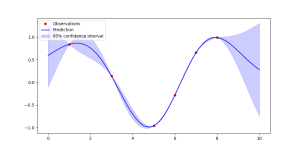
-
This reply was modified 3 months ago by Wolf.
-
This reply was modified 3 months ago by Wolf.
-
This reply was modified 3 months ago by yRocket.
-
This reply was modified 3 months ago by yRocket.
-
This reply was modified 3 months ago by yRocket.
-
This reply was modified 3 months ago by yRocket.
A Gaussian Process is a distribution over functions
Think of a Gaussian Process (GP) as the ultimate “lazy” version of machine learning. Instead of searching for a single best function to fit your data, a GP considers all possible functions that could fit and assigns a probability to each one.
For an AI learner, the most intuitive definition is: A Gaussian Process is a distribution over functions.
1. The Core Intuition
In standard linear regression, you find specific weights $w$ to define a line $y = wx + b$. In a GP, we don’t pick weights. Instead, we assume that any collection of points we pick from our function follows a Multivariate Normal Distribution.
If you have a set of input points $X = {x_1, x_2, …, x_n}$, the GP assumes the function values $f(X) = [f(x_1), f(x_2), …, f(x_n)]^T$ are distributed as:
$$f(X) \sim \mathcal{N}(\mu(X), K(X, X))$$
Where:
* $\mu(X)$: The Mean Function (usually assumed to be 0 for simplicity).
* $K(X, X)$: The Covariance Matrix (or Kernel), which defines the “shape” and smoothness of the functions.
2. The Power of the Kernel
The Kernel Function $k(x, x’)$ is the heart of a GP. It tells the model: “If input $x$ and $x’$ are close to each other, their output values $f(x)$ and $f(x’)$ should also be close.”
A common choice is the Squared Exponential (RBF) Kernel:
$$k(x, x’) = \sigma^2 \exp\left(-\frac{|x – x’|^2}{2\ell^2}\right)$$Parameter Role $\sigma$ Scale: How far the function moves vertically from the mean. $\ell$ Length-scale: How “wiggly” or smooth the function is horizontally.
3. Making Predictions (Inference)
When we have training data $(X, f)$ and want to predict the value $f_{\ast}$ at a new point $x_{\ast}$, we look at the Joint Distribution:
$$\begin{pmatrix} f \cr f_{\ast} \end{pmatrix} \sim \mathcal{N}\left( \mathbf{0}, \begin{pmatrix} K(X, X) & K(X, x_{\ast}) \cr K(x_{\ast}, X) & K(x_{\ast}, x_{\ast}) \end{pmatrix} \right)$$
Through the magic of Gaussian conditioning, the predicted distribution for $f_{\ast}$ is:
$$\bar{f}_{\ast} = K(x_{\ast}, X) K(X, X)^{-1} f$$
$$Var(f_{\ast}) = K(x_{\ast}, x_{\ast}) – K(x_{\ast}, X) K(X, X)^{-1} K(X, x_{\ast})$$Note: The prediction isn’t just a single number; it’s a mean $\bar{f}_{\ast}$ (the best guess) and a variance (the uncertainty). As you move further from training data, the variance increases, telling you the model is less confident.
4. Key Advantages for AI
- Uncertainty Quantification: It tells you what it doesn’t know. This is crucial for safety-critical AI and Bayesian Optimization.
- Non-parametric: The model complexity grows with the data; you don’t have to pre-define the number of parameters.
- Small Data King: GPs perform exceptionally well when you have very few data points (unlike Deep Learning).
Summary Comparison
Feature Linear Regression Gaussian Process Output Single Value Probability Distribution | Uncertainty Form Fixed ($y = mx + b$) Flexible (Defined by Kernel) Complexity $O(n)$ $O(n^3)$ (Can be slow for huge datasets) -
This reply was modified 3 months ago by Wolf.
From MVN to Gaussian Processes and Kalman Filters
The marginal and conditional properties of the MVN are the “secret sauce” behind some of the most powerful algorithms in AI. Let’s look at how they power Gaussian Processes (GPs) and Kalman Filters.
1. Gaussian Processes (GPs): Predicting the Unknown
A Gaussian Process is essentially an MVN with infinite dimensions. We treat a function $f(x)$ as a collection of random variables, any finite number of which have a joint Gaussian distribution.
How it uses MVN Properties:
When we “train” a GP, we aren’t actually training weights like a Neural Network. Instead, we use the Conditional Distribution formulas we discussed earlier.
- The Setup: We have observed data points $X_{train}$ (with values $y_{train}$) and we want to predict the values $y_{test}$ at new locations $X_{test}$.
- The Joint Distribution: We define a joint MVN between the knowns and unknowns:
$$\begin{pmatrix} y_{train} \cr y_{test} \end{pmatrix} \sim \mathcal{N} \left( \mathbf{0}, \begin{pmatrix} K(X_{train}, X_{train}) & K(X_{train}, X_{test}) \cr K(X_{test}, X_{train}) & K(X_{test}, X_{test}) \end{pmatrix} \right)$$
(Where $K$ is the kernel/covariance function.) - The Inference: To get the prediction, we simply calculate the Conditional Distribution $p(y_{test} | y_{train})$.
The “Mean” formula gives us our prediction, and the “Covariance” formula gives us the Uncertainty (the shaded area in GP plots).
2. Kalman Filters: Tracking Over Time
Kalman Filters are used in robotics and navigation (like GPS or self-driving cars) to estimate the state of a system (position, velocity) over time.
How it uses MVN Properties:
A Kalman Filter is essentially a recursive application of MVN properties, alternating between a Predict step and an Update step.
- The Predict Step (Marginalization):
We move our estimate forward in time. This is like adding Gaussian noise to our current state. Mathematically, this is related to the Marginal properties—specifically, how the sum of two Gaussians remains Gaussian. -
The Update Step (Conditioning):
We receive a new, noisy sensor measurement (e.g., a GPS ping). We “condition” our current estimate on this new evidence.- The Kalman Gain ($K$) is actually just the term $\Sigma_{12} \Sigma_{22}^{-1}$ from the MVN conditional mean formula!
- It determines how much we should trust the sensor vs. our internal model.
Comparison: GPs vs. Kalman Filters
Concept Primary MVN Tool Goal Gaussian Process Conditional Distribution Predict values at unobserved spatial locations. Kalman Filter Marginal (Predict) + Conditional (Update) Estimate hidden states in a temporal sequence. Summary for AI Learners
The beauty of the MVN is that Inference = Algebra. Because the math stays Gaussian after marginalizing and conditioning, these models can provide exact solutions with closed-form equations, making them incredibly robust for uncertainty quantification.
The Precision Matrix and MVN Distributions
In high-dimensional modeling and Gaussian Graphical Models (GGMs), we often work with the Precision Matrix $\Lambda$ (also denoted as $Q$ or $K$), which is the inverse of the covariance matrix:
$$\Lambda = \Sigma^{-1} = \begin{pmatrix} \Lambda_{11} & \Lambda_{12} \cr \Lambda_{21} & \Lambda_{22} \end{pmatrix}$$
While the covariance matrix $\Sigma$ tells us about marginal relationships, the precision matrix $\Lambda$ tells us about conditional relationships.
1. Conditional Distribution via Precision
One of the primary advantages of the precision matrix is that the conditional distribution formulas become much simpler. If we want the distribution of $X_1$ given $X_2$, the parameters are:
- Conditional Covariance: $\bar{\Sigma} = \Lambda_{11}^{-1}$
- Conditional Mean: $\bar{\mu} = \mu_1 – \Lambda_{11}^{-1} \Lambda_{12} (x_2 – \mu_2)$
Why this matters: In the covariance form, we had to compute a Schur complement. In the precision form, the conditional covariance is just the inverse of the top-left block.
2. Marginal Distribution via Precision
Conversely, finding the marginal distribution becomes harder with the precision matrix. To find the marginal of $X_1$, we must compute the Schur complement of the precision matrix:
- Marginal Covariance: $\Sigma_{11} = (\Lambda_{11} – \Lambda_{12} \Lambda_{22}^{-1} \Lambda_{21})^{-1}$
3. The “Zero” Property (Conditional Independence)
This is the most critical concept for AI learners. There is a beautiful duality between $\Sigma$ and $\Lambda$:
Matrix Entry Value Meaning Covariance ($\Sigma$) $\Sigma_{ij} = 0$ $X_i$ and $X_j$ are marginally independent. Precision ($\Lambda$) $\Lambda_{ij} = 0$ $X_i$ and $X_j$ are conditionally independent given all other variables. Numerical Example (Revisited)
Recall our Math ($X_1$) and Physics ($X_2$) example where $\Sigma = \begin{pmatrix} 100 & 80 \cr 80 & 100 \end{pmatrix}$. Let’s find $\Lambda$:
$$\det(\Sigma) = (100 \times 100) – (80 \times 80) = 10000 – 6400 = 3600$$
$$\Lambda = \frac{1}{3600} \begin{pmatrix} 100 & -80 \cr -80 & 100 \end{pmatrix} = \begin{pmatrix} 0.0278 & -0.0222 \cr -0.0222 & 0.0278 \end{pmatrix}$$
- The off-diagonal elements are non-zero, which confirms that Math and Physics scores are conditionally dependent.
- If we added a third variable, Study Hours ($X_3$), and found that $\Lambda_{12}$ (Math-Physics) became zero while $\Lambda_{13}$ and $\Lambda_{23}$ were non-zero, it would mean Math and Physics are only related because they both depend on Study Hours.
Summary Table
Feature Covariance Matrix $\Sigma$ Precision Matrix $\Lambda$ Marginals Easy (extract sub-matrix) Hard (Schur complement) Conditionals Hard (Schur complement) Easy (extract sub-matrix) Interpretation Marginal correlation Partial correlation / Direct links Graph View Dense connections Sparse connections (edges)
Numerical Example: 2D Multivariate Normal
Let’s walk through a concrete example. Imagine we have a 2D Gaussian distribution representing the relationship between a student’s Math Score ($X_1$) and Physics Score ($X_2$).
1. The Joint Distribution
Suppose the scores are distributed as follows:
$$X = \begin{pmatrix} X_1 \cr X_2 \end{pmatrix} \sim \mathcal{N} \left( \begin{pmatrix} 70 \cr 75 \end{pmatrix}, \begin{pmatrix} 100 & 80 \cr 80 & 100 \end{pmatrix} \right)$$
Here, the mean math score is 70, the mean physics score is 75, and they have a strong positive covariance of 80 (indicating that students who do well in math usually do well in physics).
2. Finding the Marginal
If we only care about the Math Score ($X_1$) and ignore the physics score entirely, we look at the first row/column of our parameters:
- Marginal Mean: $\mu_1 = 70$
- Marginal Variance: $\Sigma_{11} = 100$
Thus, $p(X_1) = \mathcal{N}(70, 100)$. The standard deviation is $\sqrt{100} = 10$.
3. Finding the Conditional
Now, suppose we observe that a specific student scored a 90 in Physics ($x_2 = 90$). How does this change our prediction for their Math Score ($X_1$| $X_2 = 90$)?
Step A: Calculate the New Mean ($\bar{\mu}$)
We use the formula: $\bar{\mu} = \mu_1 + \Sigma_{12} \Sigma_{22}^{-1} (x_2 – \mu_2)$
- Difference from mean: $(x_2 – \mu_2) = (90 – 75) = 15$.
- Regression Coefficient: $\Sigma_{12} \Sigma_{22}^{-1} = 80 / 100 = 0.8$.
- Update: $\bar{\mu} = 70 + 0.8(15) = 70 + 12 = 82$.
The expected math score jumped from 70 to 82 because we saw a high physics score.
Step B: Calculate the New Variance ($\bar{\Sigma}$)
We use the formula: $\bar{\Sigma} = \Sigma_{11} – \Sigma_{12} \Sigma_{22}^{-1} \Sigma_{21}$
- Reduction Term: $80 \times (1/100) \times 80 = 64$.
- Update: $\bar{\Sigma} = 100 – 64 = 36$.
The uncertainty (variance) dropped from 100 to 36. Our new standard deviation is only 6, meaning we are much more confident in our prediction of 82 than we were before we knew the physics score.
Summary of Results
Distribution Mean ($\mu$) Variance ($\Sigma$) Interpretation Marginal ($X_1$) 70 100 General population math performance. Conditional ($X_1 | 90$) 82 36 Math performance for high-achieving physics students. Notice how the conditional distribution is “tighter” and shifted toward the observed evidence.
-
This reply was modified 2 months, 4 weeks ago by
-
AuthorPosts